| A good example of the use of the data (A, B
and C) in aircraft design is given in the case study described in Chapter 16 of the book.
This study is concerned with the design of a small regional jet to replace ageing aircraft
currently used by airlines. Although these old aircraft are relatively cheap to buy (or
lease) they are expensive to operate due to the old technologies used in their original
manufacture. The study was undertaken to investigate the feasibility of designing a 70
seat aircraft incorporating advanced technology in airframe and engine designs. The description below shows how the study used data from this
Website to progress the design. The table and figure numbers refer to Chapter 16 of the
book.

Searching Data A gives the current/existing aircraft type
in the 70 to 100 seat size (Table 16.1) that are currently used for regional services.
Published airline schedules were studied to provide a list of city airport pairs typical
of such services. Data C was used to determine the stage length (great circle distance)
between each city pair (Table 16.2). These distances were compared to the aircraft design
ranges for the specimen aircraft types (Table 16.1). Data A also provided data on cruise
speed and cruise altitude (Table 16.3) and field performance (Table 16.4) for the ten
specimen aircraft. This data was used to fix the initial operational specification for the
aircraft. To check the validity of the choice of field length, all UK, French and German
airfields in Data C were analysed to provide a cumulative frequency curve (Figure 16.1)
for the available runway lengths. The chosen aircraft field length shows that over 70% of
these airfields will be suitable. To assist with technical (mass, aerodynamics and
performance) estimates for the case study, Data A was used to produce graphs for empty
mass ratio against aircraft maximum take-off mass (Figure 16.2) and lift to drag ratio
against wing loading (Figure 16.3) for the specimen aircraft. Aircraft layout and
geometrical decisions were supported by comparing wing layout, fuselage geometry (seat
layout and overall diameter) (Table 16.6) and tail sizes (area ratios and tail volume
coefficients) (Table 16.7 for horizontal tail and Table 16.8 for vertical tail) from Data
A. Engine details for typical engines used on the specimen aircraft was found from Data B
and typical engine performance charts and scaling rules found from Chapter 9 of the book.
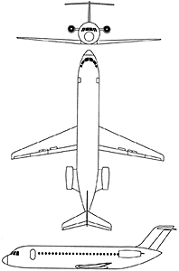
The case study shows how the initial decisions on aircraft
configuration were modified by parametric analysis to produce an ‘optimum’
layout. The final design is shown below.
Fig. 16.9

The ‘stubby’ appearance of the fuselage on this
layout results from the provision of a more comfortable fuselage/cabin layout than is
usual for this class of aircraft. This configuration will allow a fuselage stretch to 100
seats for future development of the aircraft type. The relatively small wing planform is a
consequence of the efficient aerodynamic design and the high strength materials used. The
concluding part of Chapter 16 describes the final design in detail.
Suggested Applications

These are some suggested applications for the book.
Example 1 (Flaps)

In selecting the type of flap and its geometry for a
projected aircraft it is useful to understand what previous/existing aircraft have used
and achieved. Data A can be interrogated to show the type of flap used on specimen
aircraft. A graph showing values of aircraft maximum lift coefficient against wing
sweepback angle is shown in Chapter 6 (Figure 6.11, page 118), and further details are
given in Chapter 8 (pages 167-9).
Example 2 (Mass estimation)

To determine the mass components for the initial estimation
of aircraft maximum take-off mass (MTOM) it is necessary to assume a value for the
aircraft empty mass fraction. To assist in this process it is helpful to plot this ratio
against MTOM using data of specimen aircraft taken from Data A. Such a plot is shown in
Chapter 7 (Figure 7.3, page 130).
Example 3 (Fuel mass)

The equation used to predict the fuel mass ratio for a
specified range of duration requires a knowledge of the engine specific fuel consumption
(sfc) and aircraft lift to drop ratio (L/D) as described on page 131. Data B shows
published volumes of sfc for typical engines and this can be related to the cruise
conditions (speed and height) using the generalised engine performance charts in Chapter 9
(pages 203-213). The aircraft L/D ratio can be determined for specimen aircraft from Data
A.
Example 4 (Engine Size)

To size the engine for a particular project aircraft it is
useful to use the engine data (from Data B) for specimen engines of the same
operating/design conditions (e.g. by-pass ratio). This can then be scaled to determine
geometry and performance for your aircraft using the charts and rules given in Chapter 9
(page 201 onwards).
Example 5 (Unit Conversions)

Although most technical analysis on a project will be done
using SI units it is necessary to use Data D and E to convert values to units that are
commonly used and understood in industry, or to transfer published data into SI units for
use in your design work. An example of such complications is given on page 318 of the
book. Here it is necessary to convert aviation fuel density and volume from SI units to US
gallons to predict the cost of fuel used in the flight (e.g. US$ per hour). |