Chapter 05
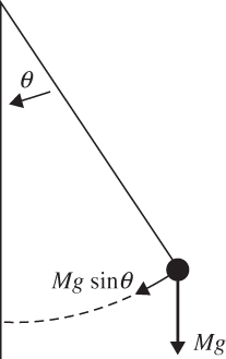
FIGURE 5.1 A simple pendulum.
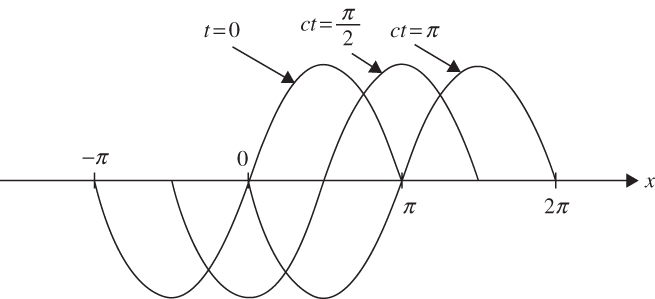
FIGURE 5.2 A sinusoidal wave traveling in the positive x direction at speed c. (Wave number is assumed to be unity.)
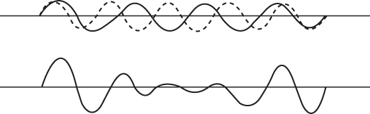
FIGURE 5.3 Wave groups formed from two sinusoidal components of slightly different wavelengths. For nondispersive waves, the pattern in the lower part of the diagram propagates without change of shape. For dispersive waves, the shape of the pattern changes in time.
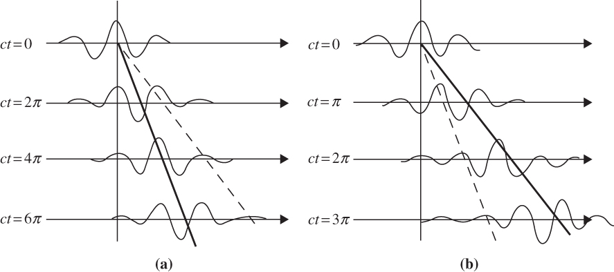
FIGURE 5.4 Schematic showing propagation of wave groups: (a) group velocity less than phase speed and (b) group velocity greater than phase speed. Heavy lines show group velocity, and light lines show phase speed.
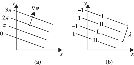
FIGURE 5.5 Two-dimensional plane wave at a fixed time: (a) phase angle, Φ, and (b) phase, eiΦ. Wavelength is denoted λ. Note that if v> 0, the wave travels in the direction of the wave vector, ∇Φ.
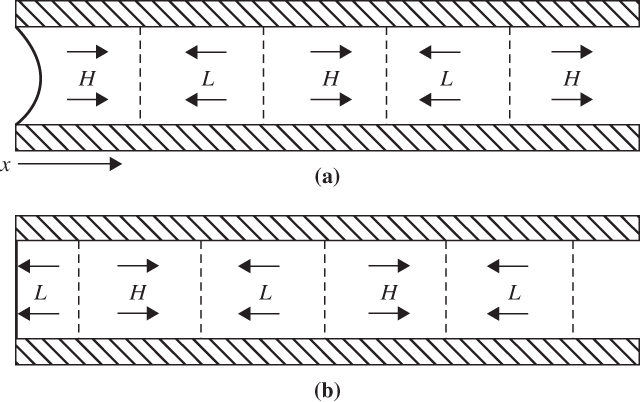
FIGURE 5.6 Schematic diagram illustrating the propagation of a sound wave in a tube with a flexible diaphragm at the left end. Labels H and L designate centers of high- and low-perturbation pressure. Arrows show velocity perturbations. The situation one-quarter period (b) later than in (a) for propagation in the positive x direction.
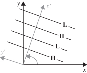
FIGURE 5.7 Coordinate rotation to align the y axis with wave fronts so that l = 0.
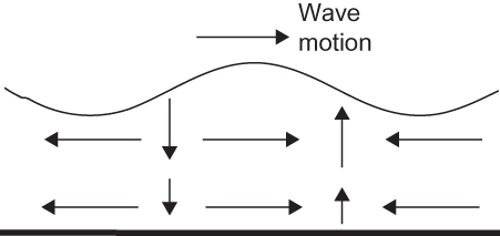
FIGURE 5.8 Depiction of shallow water gravity wave height and velocity fields for the case where the coordinates have been rotated as shown in Figure 5.7.
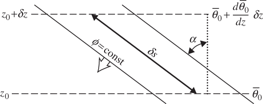
FIGURE 5.9 Parcel oscillation path (heavy arrow) for pure gravity waves with phase lines tilted at an angle α to the vertical.
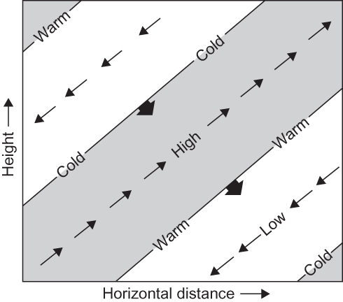
FIGURE 5.10 Idealized cross-section showing phases of pressure, temperature, and velocity perturbations for an internal gravity wave. Thin arrows indicate the perturbation velocity field; blunt solid arrows, the phase velocity. Shading shows regions of upward motion.
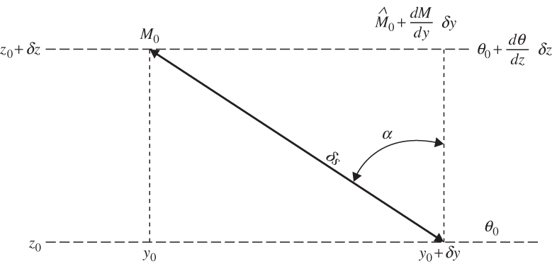
FIGURE 5.11 Parcel oscillation path in the meridional plane for an inertia–gravity wave. (See text for definition of symbols.)
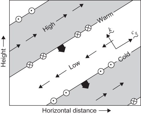
FIGURE 5.12 Vertical section in a plane containing the wave vector k showing the phase relationships among velocity, geopotential, and temperature fluctuations in an upward propagating inertia–gravity wave with m < 0, v > 0, and f > 0 (Northern Hemisphere). Thin sloping lines denote the surfaces of constant phase (perpendicular to the wave vector), and thick arrows show the direction of phase propagation. Thin arrows show the perturbation zonal and vertical velocity fields. Meridional wind perturbations are shown by arrows pointed into the page (northward) and out of the page (southward). Note that the perturbation wind vector turns clockwise (anticyclonically) with height. (After Andrews et al., 1987.)
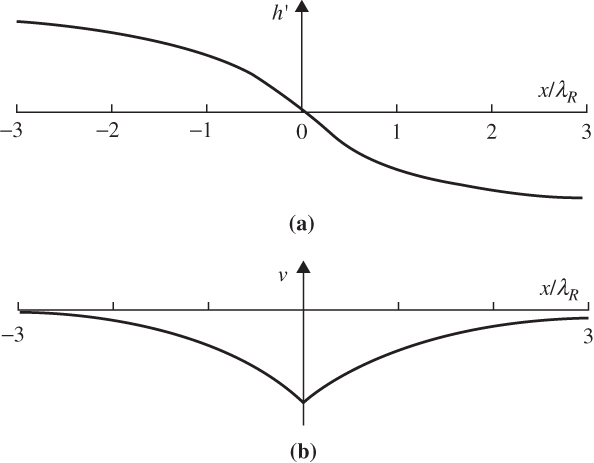
FIGURE 5.13 The geostrophic equilibrium solution corresponding to adjustment from the initial state defined in (5.97). (a) Final surface elevation profiles and (b) the geostrophic velocity profile in the final state. (After Gill, 1982.)
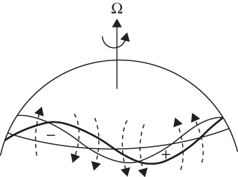
FIGURE 5.14 Perturbation vorticity field and induced velocity field (dashed arrows) for a meridionally displaced chain of fluid parcels. The heavy wavy line shows original perturbation position; the light line shows westward displacement of the pattern due to advection by the induced velocity.
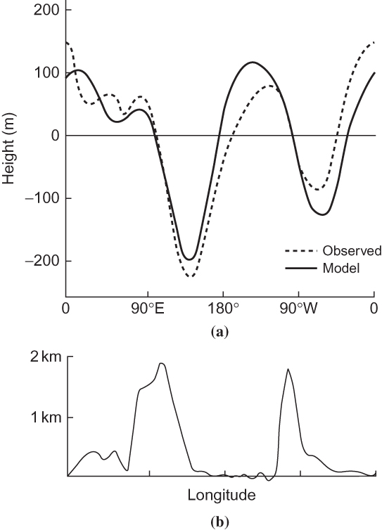
FIGURE 5.15 (a) Longitudinal variation of the disturbance in geopotential height (≡ f0ψ/g) in the Charney–Eliassen model for the parameters given in the text (solid line) compared with the observed 500-hPa height perturbations at 45°N in January (dashed line). (b) Smoothed profile of topography at 45°N used in the computation. (After Held, 1983.)