Chapter 06
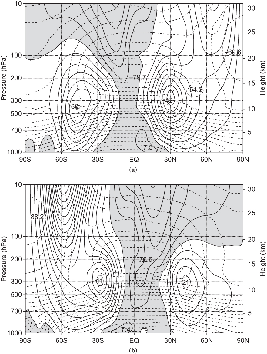
FIGURE 6.1 Meridional cross-sections of longitudinally and time-averaged zonal wind (solid contours, interval of 5 m s-¹) and temperature (dashed contours, interval of 5 K) for December– February (a) and June–August (b). Easterly winds are shaded and 0°C isotherm is darkened. Wind maxima shown in m s-¹, temperature minima shown in °C. (Based on NCEP/NCAR reanalyses; after Wallace, 2003.)
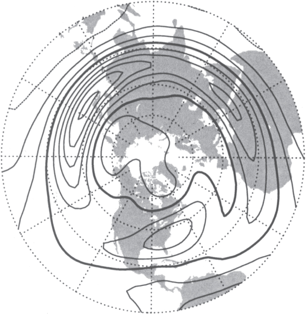
FIGURE 6.2Mean zonal wind at the 200-hPa level for December through February, averaged for years 1958–1997. Contour interval 10 m s-¹ (heavy contour, 20 m s-¹). (Based on NCEP/NCAR reanalyses; after Wallace, 2003.)
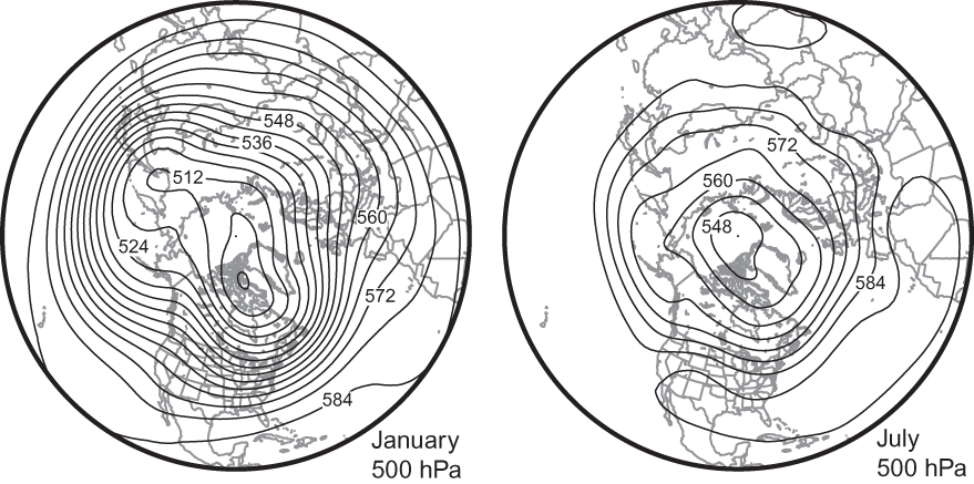
FIGURE 6.3 Mean 500-hPa geopotential height contours in January (left) and July (right) in the Northern Hemisphere (30-year average). Geopotential height contours are shown every 60 meters. (Adapted from NOAA/ESRL http://www.esrl.noaa.gov/psd/.)
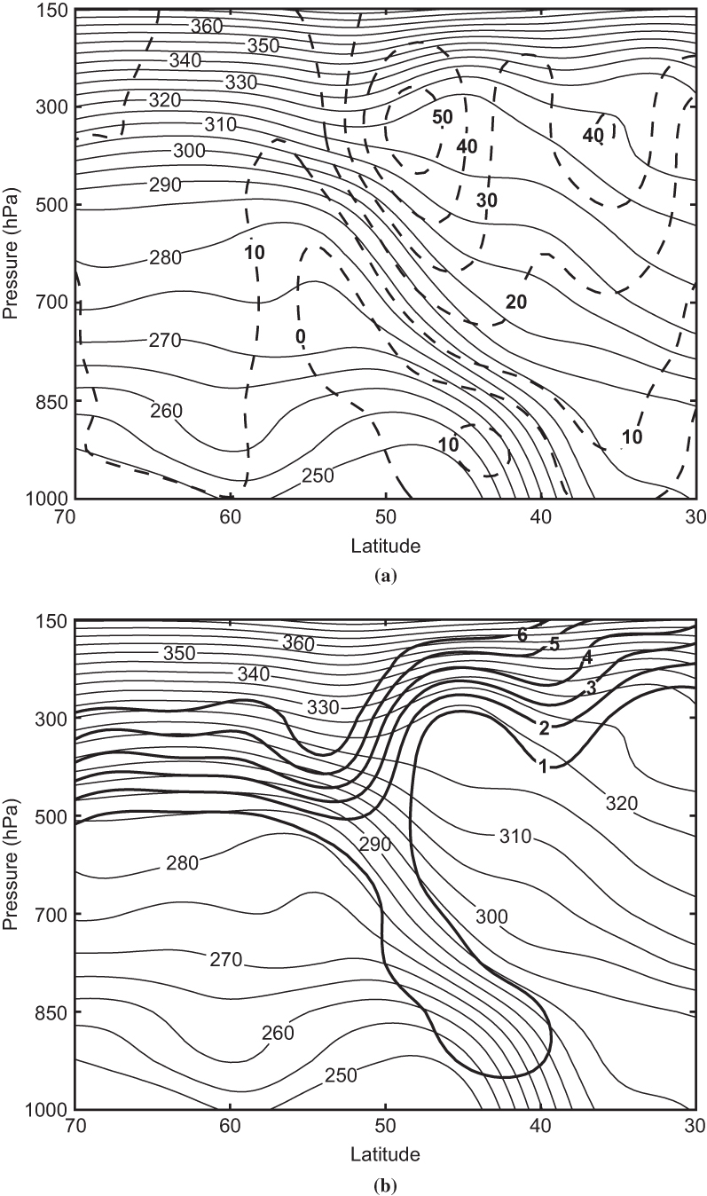
FIGURE 6.4 Latitude–height cross-sections through a cold front at 80W longitude on 2000 UTC January 14, 1999. (a) Potential temperature contours (thin solid lines, K) and zonal wind isotachs (dashed lines, m s-¹). (b) Thin solid contours as in (a), heavy dashed contours, Ertel potential vorticity labeled in PVU (1-PVU = 10–6 K kg-¹ m² s-¹).
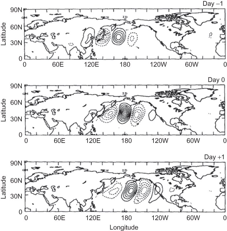
FIGURE 6.5 Linear regression of the meridional wind relative to the base point at 40°N, 180°W. Contours are shown every 2 m s-¹ with negative values dashed. The top, middle, and bottom panels show lags of –1, 0, and +1 days, respectively, relative to the base point, which reveals the motion of the baroclinic waves across the North Pacific ocean. (After Chang, 1993. Copyright © American Meteorological Society. Reprinted with permission.)
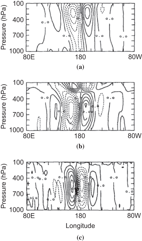
FIGURE 6.6 Linear regression is shown on the longitude–height plane of (a) geopotential height (b) temperature, and (c) vertical motion (ω) relative to the meridional wind at the base point located at 300 hPa, 40°N, and 180°W. Contours are shown every 20 m for geopotential height, 0.5 K for temperature, and 0.02 Pa s-¹ for vertical motion, with negative values dashed. (After Chang, 1993. Copyright © American Meteorological Society. Reprinted with permission.) The vertical structure of baroclinic waves is revealed: westward tilt with height for geopotential height anomalies, eastward tilt with height for temperature, and rising motion eastward of the geopotential height trough axis.
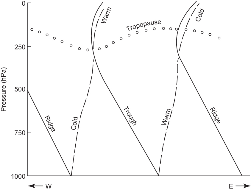
FIGURE 6.7 West–east cross-section through a developing baroclinic wave. Solid lines are trough and ridge axes; dashed lines are axes of temperature extrema; the chain of open circles denotes the tropopause.
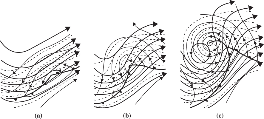
FIGURE 6.8 Schematic 500-hPa contours (heavy solid lines), 1000-hPa contours (thin lines), and 1000–500-hPa thickness (dashed lines) for a developing extratropical cyclone at three stages of development: (a) incipient development stage, (b) rapid development stage, and (c) occlusion stage. (After Palmén and Newton, 1969.)
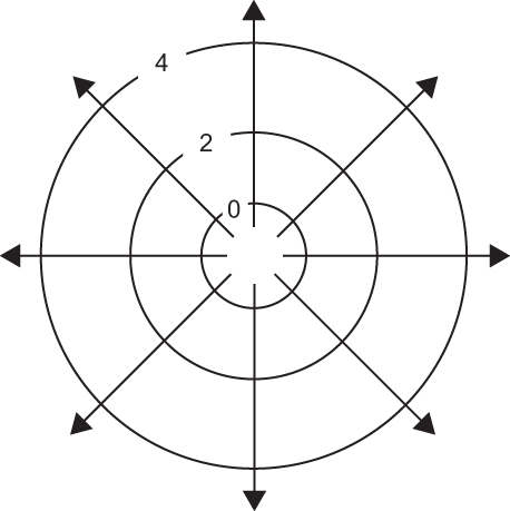
FIGURE 6.9 Illustration of the gradient operator for a scalar function, Φ. The gradient of Φ, a vector field, is illustrated by arrows that are directed toward larger values and orthogonal to lines of constant Φ. The Laplacian is given by the divergence of the gradient, which is a local maximum near the local minimum in Φ.
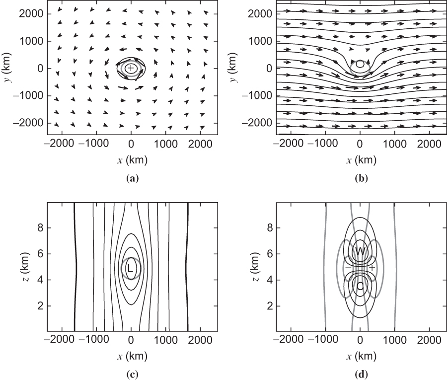
FIGURE 6.10 Inversion of an idealized localized blob of QG PV having a magnitude of 2 PVU embedded in a jet stream consisting of a westerly wind increasing linearly with height. (a) PV contours at altitude of 5 km are shown every 0.5 PVU; wind induced by the PV anomaly is shown by arrows, with a maximum wind speed of 22 m s-¹; (b) pressure contours every 42 hPa (equivalent to 60-m height contours on an isobaric surface) and full wind vectors (wind due to the PV anomaly plus the westerly jet), with a maximum wind speed of 36 m s-¹; (c) anomaly pressure every 21 hPa (equivalent to 30-m height contours) with bold zero contour; and (d) meridional wind every 6 m s-¹ and potential-temperature anomalies every 2 K ("W" and "C"imply "warm" and "cold" values). In (a) through (c), the 1-PVU QG PV contour is denoted by the thick gray line.
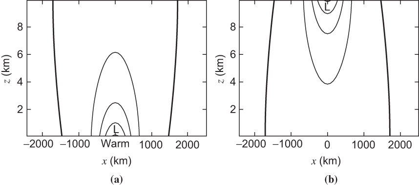
FIGURE 6.11 Pressure contours associated with (a) surface warm anomaly and (b) tropopause cold anomaly. Pressure is contoured every 21 hPa (equivalent to 30-m height contours) with bold zero contour. The potential temperature anomalies have an amplitude of 10 K and the same horizontal shape as the PV anomaly in Figure 6.10.
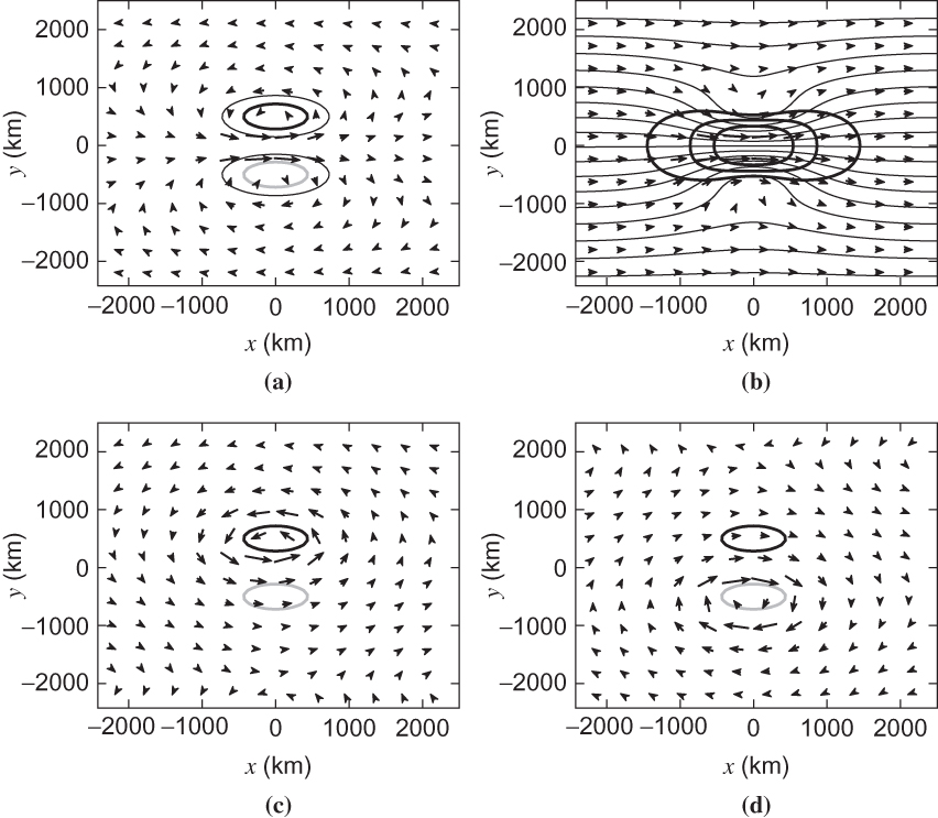
FIGURE 6.12 Idealized model of a "jet streak" as a dipole of QG PV having a magnitude of 2 PVU embedded in a jet stream consisting of a westerly wind increasing linearly with height. (a) PV contours at a height of 5 km are shown every 0.5 PVU; wind induced by the PV anomaly is shown by arrows, with a maximum wind speed of 22 m s-¹; (b) pressure contours at 5 km every 42 hPa (equivalent to 60-m geopotential height contours on an isobaric surface), full wind vectors (wind due to the PV dipole plus the westerly jet), and isotachs (20, 30, and 40 m s-¹) in thick lines; (c) wind induced by the positive anomaly; (d) wind induced by the negative PV anomaly. In (c) and (d) the –1- and 1-PVU QG PV contours are denoted by the thick gray and black lines, respectively.
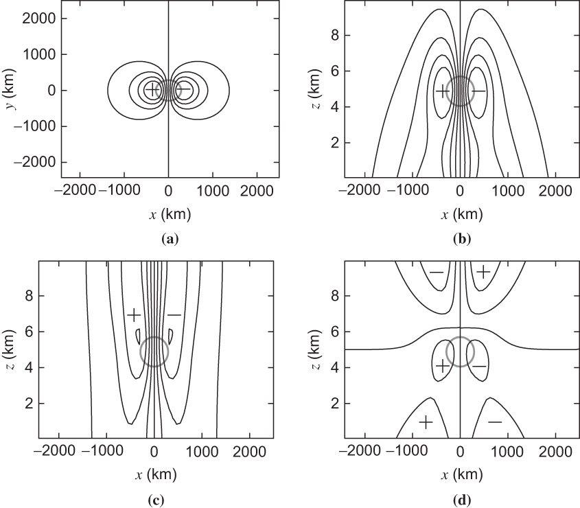
FIGURE 6.13 Pressure tendency associated with the PV blob in vertical shear shown in Figure 6.10. Pressure tendency: (a) plan view at 5-km altitude; (b) cross-section along y = 0; (c) cross-section along y = 0 of vorticity advection contribution; and (d) cross-section along y = 0 of temperature advection contribution. The sum of (c) and (d) equals (b). Pressure tendency contours are shown every 5 hPa (day)-¹, and the 1-PVU QG PV contour by a thick gray line.
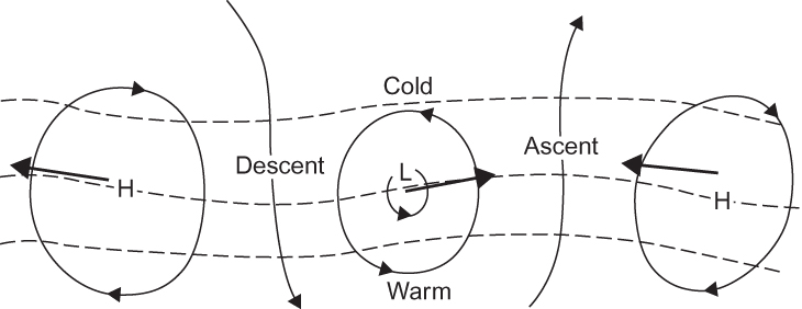
FIGURE 6.14 Q vectors (bold arrows) for an idealized pattern of isobars (solid lines) and isotherms (dashed lines) for a family of cyclones and anticyclones. (After Sanders and Hoskins, 1990.)
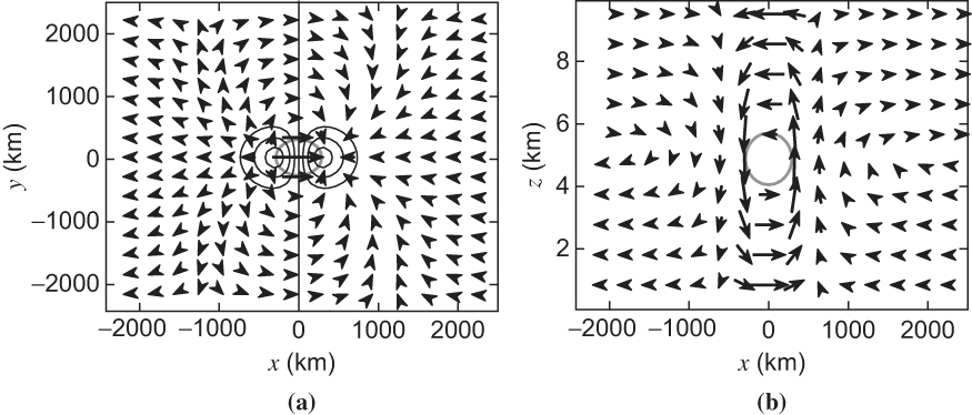
FIGURE 6.15 Vertical motion associated with the PV blob in vertical shear shown in Figure 6.10. (a) Q-vectors and contours of w every 2 cm s-¹, with rising air where Q-vectors converge; (b) vertical cross-section along y = 0 of the ageostrophic circulation (ua, w). The 1-PVU QG PV contour is shown by a thick gray line.
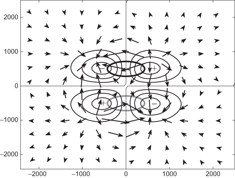
FIGURE 6.16 Vertical motion associated with the jet streak shown in Figure 6.12. Contours show vertical motion (w) at 5-km altitude every 1 cm s-¹, and arrows show the divergent ageostrophic wind. The –1- and 1-PVU QG PV contours are denoted by the thick gray and black lines, respectively.
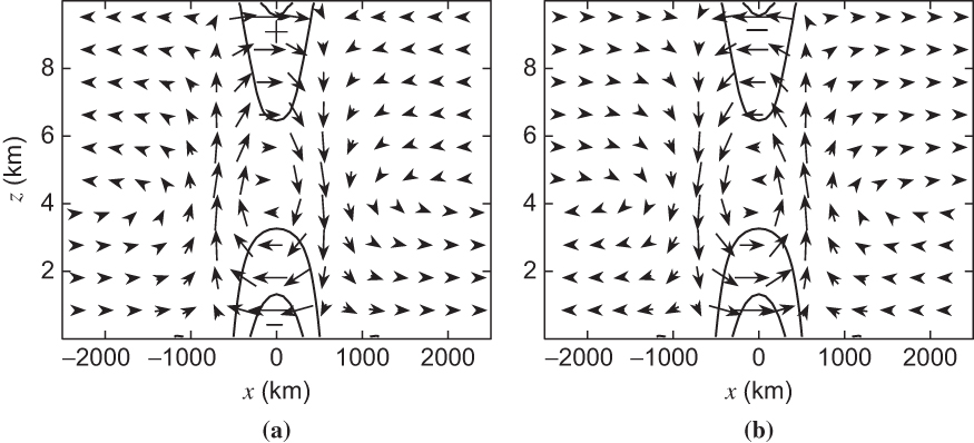
FIGURE 6.17 Vertical cross-section of ageostrophic circulation (ua, w) near the (a) jet entrance (x = –700 km) and (b) jet exit (x = 700 km) regions. Contours show the acceleration of the geostrophic zonal wind,Du/Dt , every 5 m s-¹ per hour.
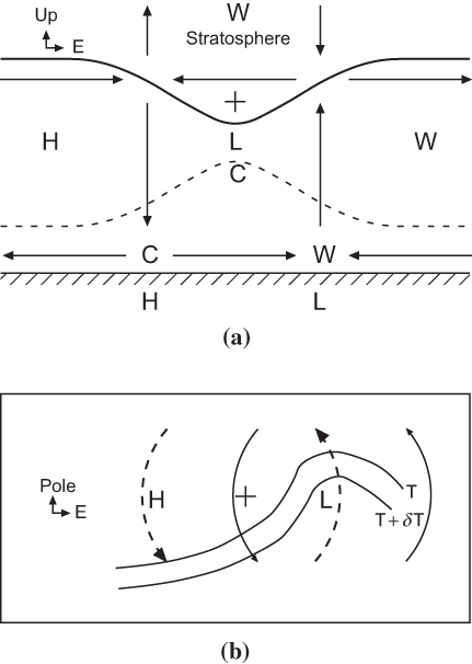
FIGURE 6.18 Schematic of quasi-geostrophic reasoning applied to extratropical cyclone development. (a) East–West vertical section showing the tropopause (thick solid line), the surface (cross-hatched line), a lower-tropospheric isentropic surface (dashed line), and the air circulations required to conserve potential vorticity for the typical case where westerly winds are increasing from the surface to the tropopause. Regions of relatively warm and cold air are given by "W" and "C," respectively, and regions of relatively low and high pressure are given by "L" and "H," respectively. (b) Horizontal plan view showing the surface isotherms (solid lines), surface wind associated with the upper-level PV disturbance (thick dashed lines with arrows), and surface wind associated with the surface cyclone (thin solid lines with arrows). In both (a) and (b), "+" shows the location of the PV disturbance due to the lowered tropopause. (From Hakim, 2002.)