Chapter 07
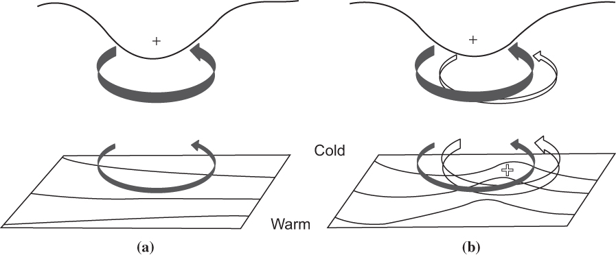
FIGURE 7.1 A schematic picture of cyclogenesis associated with the arrival of an upper-level potential vorticity perturbation over a lower-level baroclinic region. (a) Lower-level cyclonic vorticity induced by the upper-level potential vorticity anomaly. The circulation induced by the potential vorticity anomaly is shown by the solid arrows, and potential temperature contours are shown at the lower boundary. The advection of potential temperature by the induced lower-level circulation leads to a warm anomaly slightly east of the upper-level vorticity anomaly. This in turn will induce a cyclonic circulation as shown by the open arrows in (b). The induced upper-level circulation will reinforce the original upper-level anomaly and can lead to amplification of the disturbance. (After Hoskins et al., 1985.)
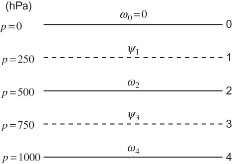
FIGURE 7.2 Arrangement of variables in the vertical for the two-level baroclinic model.
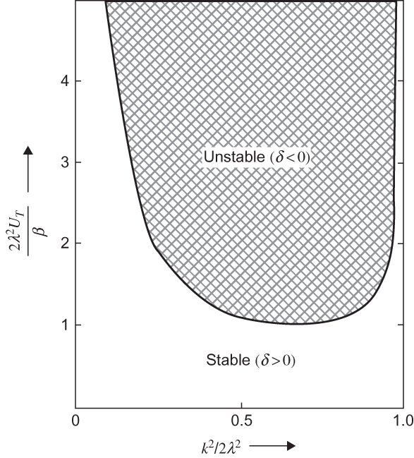
FIGURE 7.3 Neutral stability curve for the two-level baroclinic model.
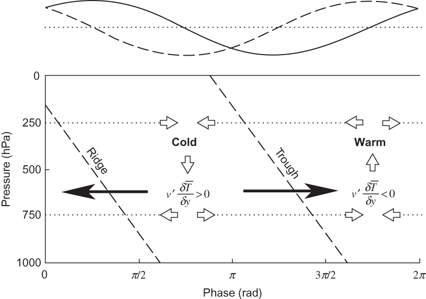
FIGURE 7.4 Structure of an unstable baroclinic wave in the two-level model.(Top) Relative phases of the 500-hPa perturbation geopotential (solid line) and temperature (dashed line). (Bottom) Vertical cross-section showing phases of geopotential, meridional temperature advection, ageostrophic circulation (open arrows), Q vectors (solid arrows), and temperature fields for an unstable baroclinic wave in the two-level model.
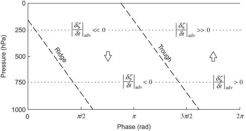
FIGURE 7.5 Vertical cross-section showing the phase of vorticity change due to vorticity advection for an unstable baroclinic wave in the two-level model.
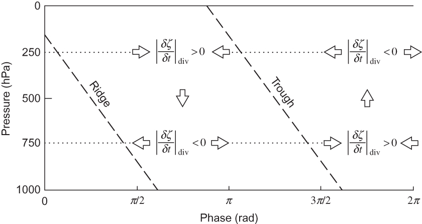
FIGURE 7.6 Vertical cross-section showing the phase of vorticity change due to divergence– convergence for an unstable baroclinic wave in the two-level model.
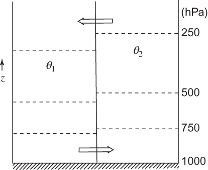
FIGURE 7.7 Two air masses of differing potential temperature separated by a vertical partition. Dashed lines indicate isobaric surfaces. Arrows show direction of motion when the partition is removed.
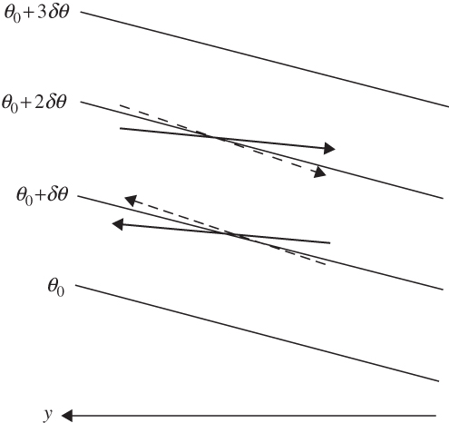
FIGURE 7.8 Slopes of parcel trajectories relative to the zonal-mean potential temperature surfaces for a baroclinically unstable disturbance (solid arrows) and for a baroclinically stable disturbance (dashed arrows).
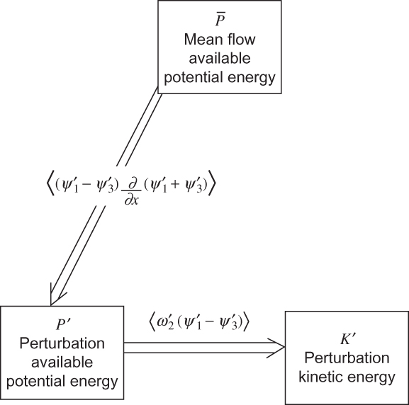
FIGURE 7.9 Energy flow in an amplifying baroclinic wave.
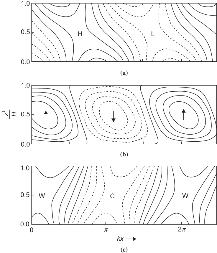
FIGURE 7.10 Properties of the most unstable Eady wave. (a) Contours of perturbation geopotential height; "H" and "L" designate ridge and trough axes, respectively. (b) Contours of vertical velocity; up and down arrows designate axes of maximum upward and downward motion, respectively. (c) Contours of perturbation temperature; "W" and "C" designate axes of warmest and coldest temperatures, respectively. In all panels 1 and 1/4 wavelengths are shown for clarity.
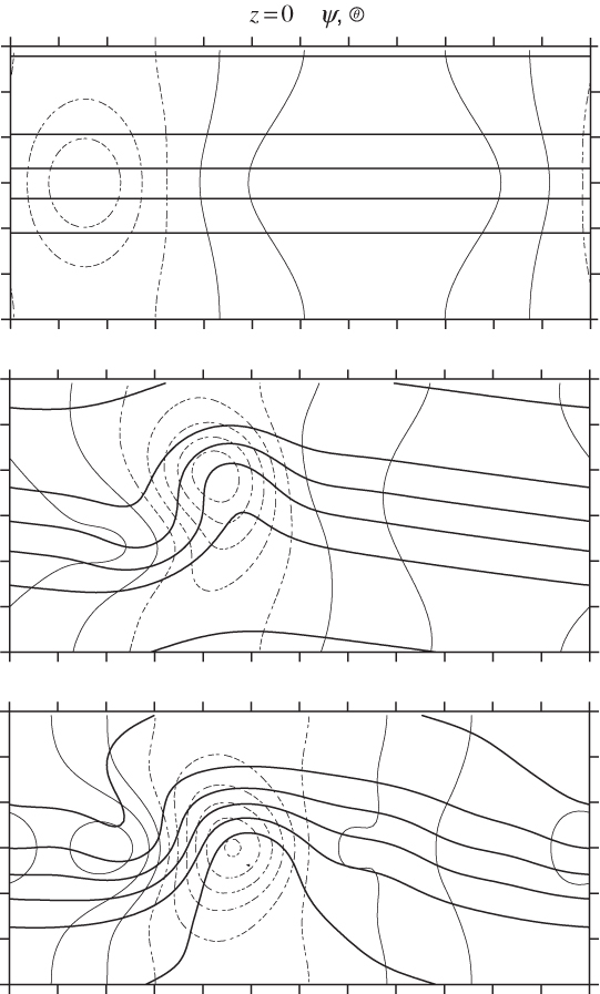
FIGURE 7.11 Development of a spatially localized disturbance in an idealized westerly jet stream. Dashed lines show pressure every 4 hPa and solid lines show potential temperature every 5 K. An initial surface disturbance (top panel) associated with an upper-level PV anomaly evolves into a well-developed extratropical cyclone 48 h later (middle panel). The linear solution for only the projection of the initial disturbance onto the unstable normal modes (bottom panel) captures most of the development of the full nonlinear solution. (Adapted from Hakim, 2000. Copyright © American Meteorological Society. Reprinted with permission.)
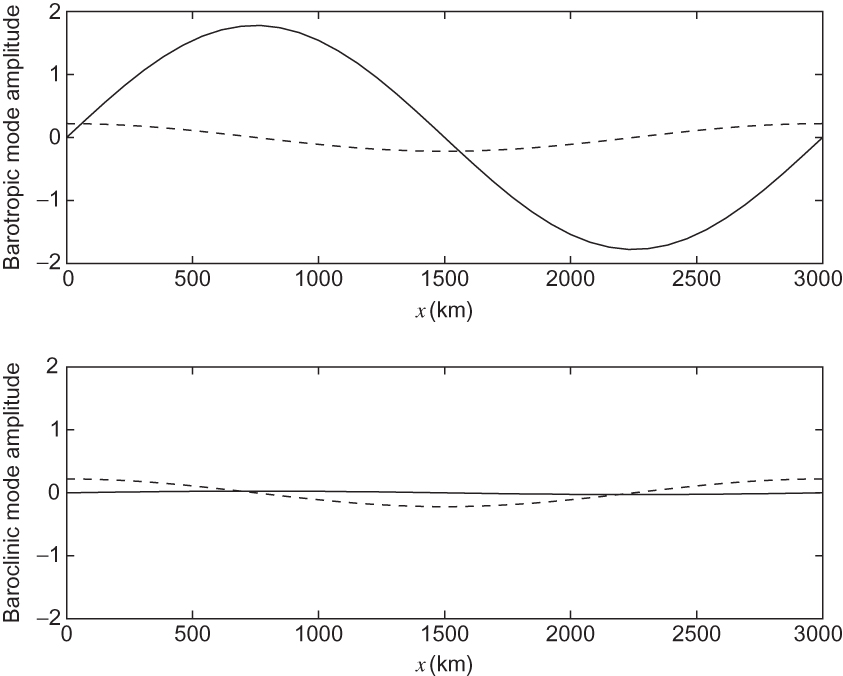
FIGURE 7.12 Zonal distribution of the amplitude of a transient neutral disturbance initially confined entirely to the upper layer in the two-layer model. Dashed lines show the initial distribution of the baroclinic and barotropic modes; solid lines show the distribution at the time of maximum amplification.
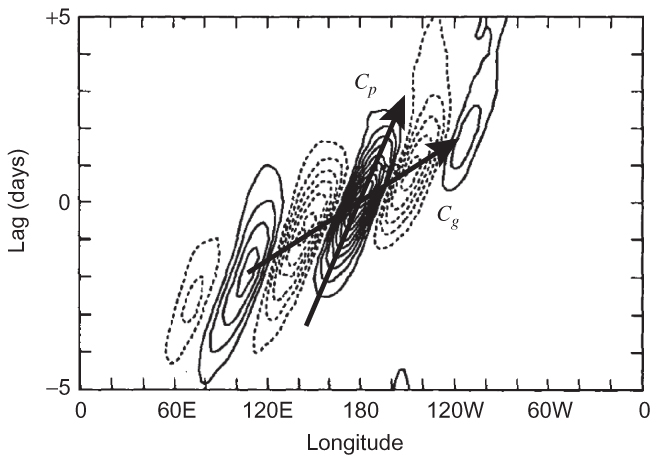
FIGURE 7.13 Time-series correlation of meridional wind as a function of longitude and time lag. Correlation is shown every 0.1 unit (i.e., a unitless number between –1 and 1), with the reference time series at 180. Results are averaged over 30 to 60° N latitude during winter. (From Chang, 1993. Copyright © American Meteorological Society. Reprinted with permission.)