Chapter 09
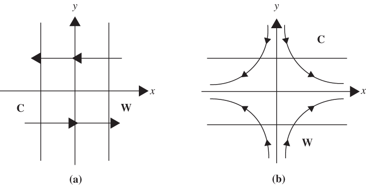
FIGURE 9.1 Frontogenetic flow configurations: (a) shows horizontal shearing deformation and (b) shows horizontal stretching deformation.
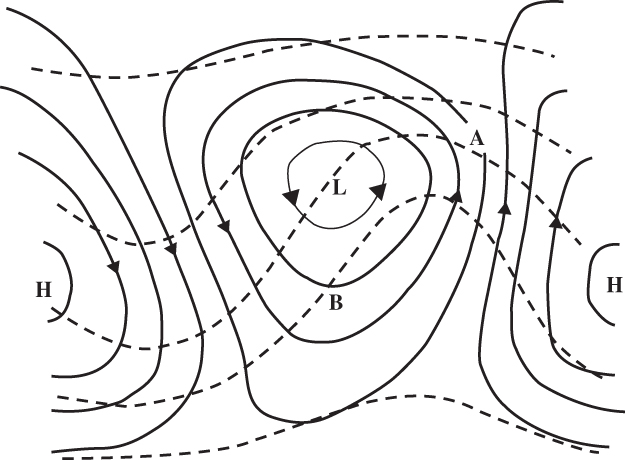
FIGURE 9.2 Schematic surface isobars (solid lines) and isotherms (dashed lines) for a baroclinic wave disturbance. Arrows show direction of geostrophic wind. Horizontal stretching deformation intensifies the temperature gradient at A, and horizontal shear deformation intensifies the gradient at B. (After Hoskins and Bretherton, 1972. Copyright © American Meteorological Society. Reprinted with permission.)
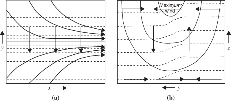
FIGURE 9.3 (a) Horizontal streamlines, isotherms, and Q-vectors in a frontogenetic confluence. (b) Vertical section across the confluence showing isotachs (solid lines), isotherms (dashed lines), and vertical and transverse motions (arrows). (After Sawyer, 1956. Copyright © The Royal Society. Reprinted with permission.)
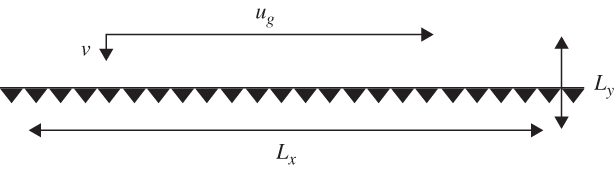
FIGURE 9.4 Velocity and length scales relative to a front parallel to the x axis.
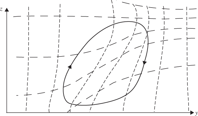
FIGURE 9.5 Relationship of the ageostrophic circulation (heavy curve with arrows) in twodimensional frontogenesis to the potential temperature field (long dashes) and absolute momentum field (short dashes). Cold air is on the right and warm air is on the left. Note the tilt of the circulation toward the cold air side and the enhanced gradients of the absolute momentum and potential temperature fields in the frontal zone.
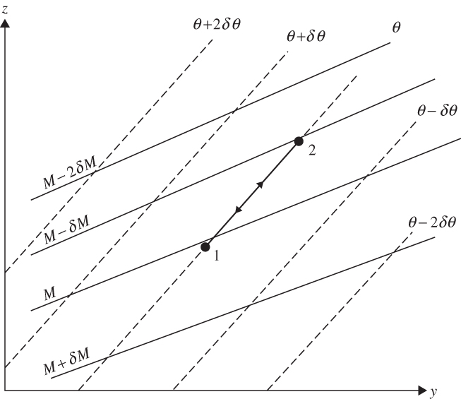
FIGURE 9.6 Cross-section showing isolines of absolute momentum and potential temperature for a symmetrically unstable basic state. Motion along the isentropic path between points labeled 1 and 2 is unstable, as M decreases with latitude along the path. See text for details.
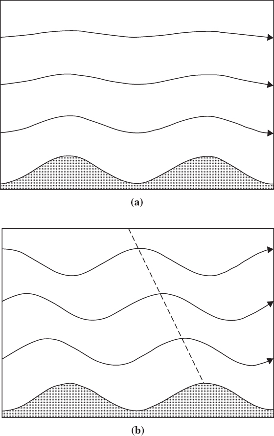
FIGURE 9.7 Streamlines in steady flow over an infinite series of sinusoidal ridges for the narrow ridge case (a) and broad ridge case (b). The dashed line in (b) shows the phase of maximum upward displacement. (From Durran, 1990. Copyright © American Meteorological Society. Reprinted with permission.)
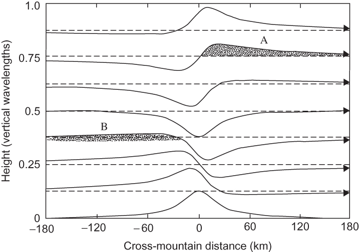
FIGURE 9.8 Streamlines of flow over a broad isolated ridge showing upstream phase tilt with height. The pattern is periodic in height, and one vertical wavelength is shown. Orographic clouds may form in the shaded areas where streamlines are displaced upward from equilibrium either upstream or downstream of the ridge if sufficient moisture is present. (After Durran, 1990. Copyright © American Meteorological Society. Reprinted with permission.)
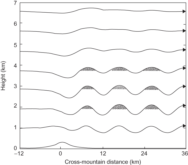
FIGURE 9.9 Streamlines for trapped lee waves generated by flow over topography with vertical variation of the Scorer parameter. Shading shows locations where lee wave clouds may form. (After Durran, 1990. Copyright © American Meteorological Society. Reprinted with permission.)
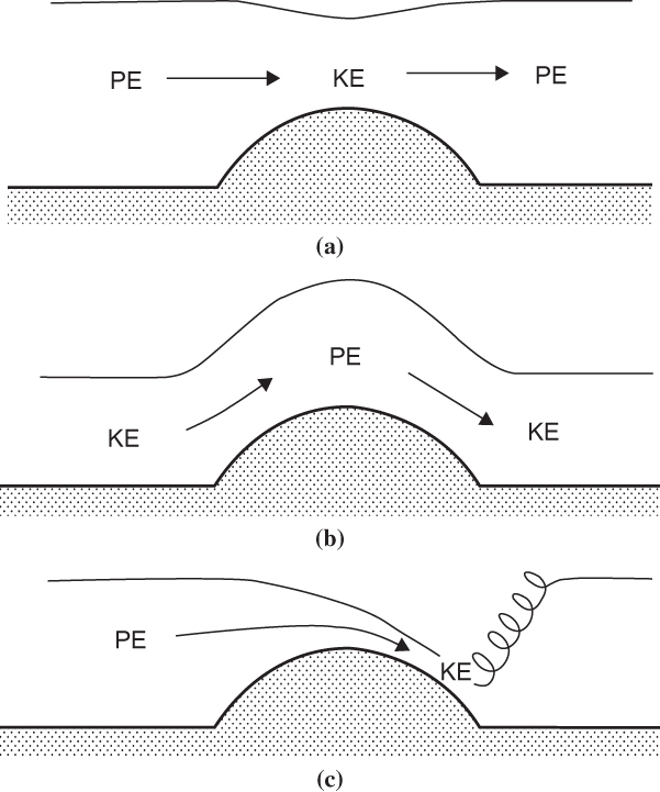
FIGURE 9.10 Flow over an obstacle for a barotropic fluid with free surface. (a) Subcritical flow (Fr > 1 everywhere). (b) Supercritical flow (Fr < 1 everywhere). (c) Supercritical flow on lee slope with adjustment to subcritical flow at hydraulic jump near base of obstacle. (After Durran, 1990. Copyright © American Meteorological Society. Reprinted with permission.)
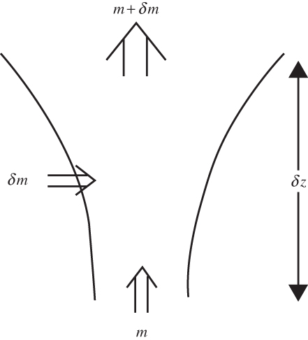
FIGURE 9.11 An entraining jet model of cumulus convection. See text for an explanation.
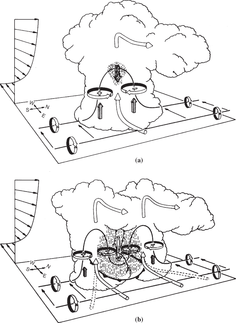
FIGURE 9.12 Development of rotation and splitting in a supercell storm with westerly mean wind shear (shown by storm relative wind arrows in the upper left corner of each panel). Cylindrical arrows show the direction of cloud relative air flow. Heavy solid lines show vortex lines with a sense of rotation shown by circular arrows. Plus and minus signs indicate cyclonic and anticyclonic rotation caused by vortex tube tilting. Shaded arrows represent updraft and downdraft growth. Vertical dashed lines denote regions of precipitation. (a) In the initial stage, the environmental shear vorticity is tilted and stretched into the vertical as it is swept into the updraft. (b) In the splitting stage, downdraft forms between the new updraft cells. The arced line with triangles in the lower middle of (b) at the surface indicates downdraft outflow at the surface. (After Klemp, 1987. Used with permission from Annual Reviews.)
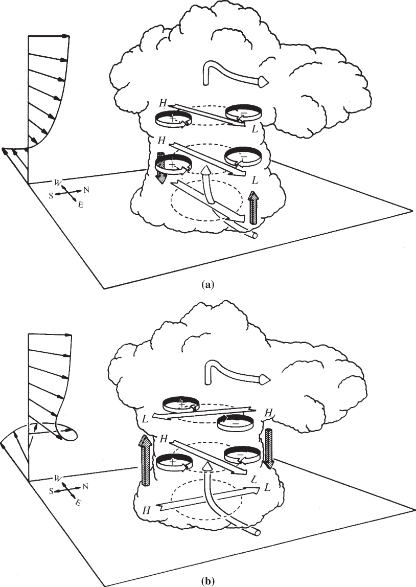
FIGURE 9.13 Pressure and vertical vorticity perturbations produced by interaction of the updraft with environmental wind shear in a supercell storm. (a) Wind shear does not change direction with height. (b) Wind shear turns clockwise with height. Broad open arrows designate the shear vectors. H and L designate high and low dynamical pressure perturbations, respectively. Shaded arrows show resulting disturbance vertical pressure gradients. (After Klemp, 1987. Used with permission from Annual Reviews.)
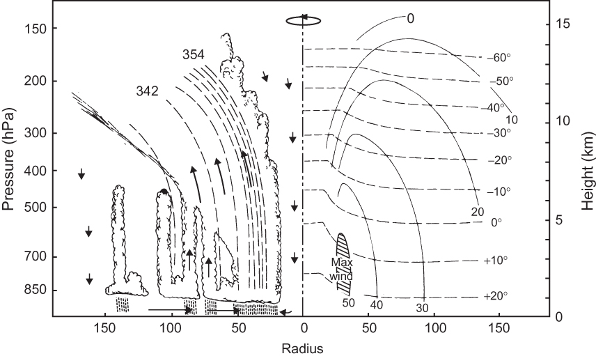
FIGURE 9.14 Schematic illustration of hurricane structure. Thin solid curves show the azimuthal wind speeds, which peak in the lower troposphere. Mainly horizontal dashed lines give the temperature field, which reflects the decrease with height in the troposphere. Mainly vertical thin dashed lines show equivalent potential temperature, which is well mixed in the eyewall. Arrows denote the secondary circulation, with radial inflow at low levels, ascent in the eyewall, and subsidence in the environment and inside the eye. (Adapted from Wallace and Hobbs, 2006.)
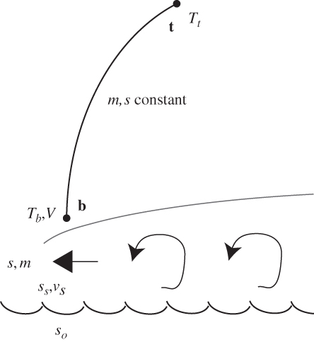
FIGURE 9.15 Essential elements of the potential intensity theory. The bold curve with endpoints b and t denotes the constant entropy and angular momentum surface along which the thermal wind equation is integrated. The curve originates at the top of the boundary layer, which is denoted by the sloping gray curve. Within the boundary layer, radial advection of entropy and angular momentum, denoted by the bold arrow (positive for angular momentum and negative for entropy) is balanced by vertical flux divergence due to turbulence, denoted by the curved arrows. At the sea surface, there exists an entropy difference between values in the atmosphere, ss and ocean, so. The surface wind speed is given by vs.
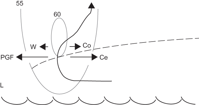
FIGURE 9.16 Illustration of unbalanced contributions to the azimuthal wind following an air parcel from the boundary layer into the free atmosphere (thick arrow) near the radius of maximum wind (isotachs of azimuthal wind speed given by gray contours in m/s). A large pressure gradient force is directed inward toward low pressure in the eye ("L"). If vertical motion is small, then the vertical advection of horizontal azimuthal momentum ("W") may be neglected, which results in a balance between the pressure gradient force and the sum of the Coriolis ("Co") and centrifugal ("Ce") forces—that is, gradient wind balance. If vertical advection is large, a stronger azimuthal wind is required to achieve balance, which yields winds stronger than that for gradient balance. In this situation, when parcels approach the level maximum wind, vertical advection approaches zero, resulting in a net outward force that decelerates the wind.
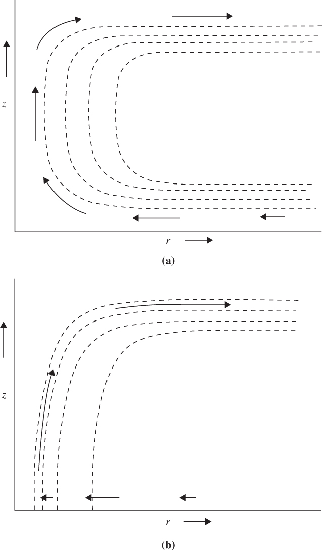
FIGURE 9.17 Meridional cross-sections showing the relationship between surfaces of constant saturation θe (dashed contours; values decreasing as r increases) and meridional circulation (arrows) in CISK (a) and WISHE (b) theories for hurricane development. (a) Frictionally induced boundary layer convergence moistens the environment and destabilizes it through layer ascent. This enables small-scale plumes to reach their levels of free convection easily and to produce cumulonimbus clouds. Diabatic heating due to the resulting precipitation drives large-scale circulation and thus maintains the large-scale convergence. (b) The saturation θe is tied to the θe of the boundary layer. The warm core occurs because enhanced surface fluxes of latent heat increase θe there. (After Emanuel, 2000.)