Chapter 10
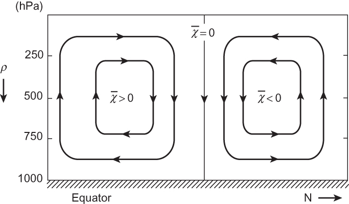
FIGURE 10.1 Relationship of the Eulerian mean meridional streamfunction to vertical and meridional motion.
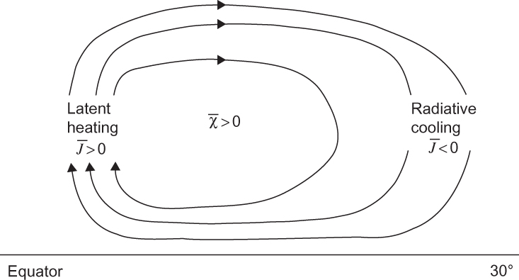
FIGURE 10.2 Schematic Eulerian mean meridional circulation showing the streamfunction for a thermally direct Hadley cell.
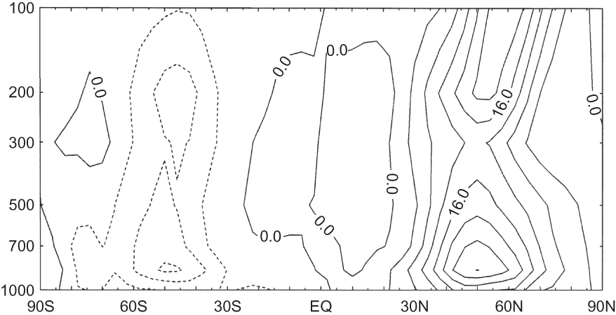
FIGURE 10.3 Observed northward eddy heat flux distribution (°Cms-¹) for Northern Hemisphere winter. (Adapted from Schubert et al., 1990.)
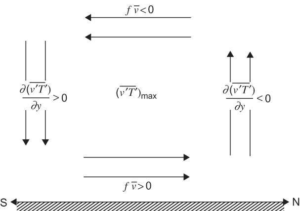
FIGURE 10.4 Schematic Eulerian mean meridional circulation forced by poleward heat fluxes.
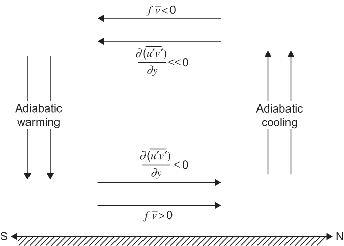
FIGURE 10.5 Schematic Eulerian mean meridional circulation forced by a vertical gradient in eddy momentum flux convergence.
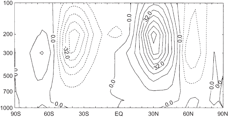
FIGURE 10.6 Observed northward eddy momentum flux distribution (m² s-²) for Northern Hemisphere winter. (Adapted from Schubert et al., 1990.)
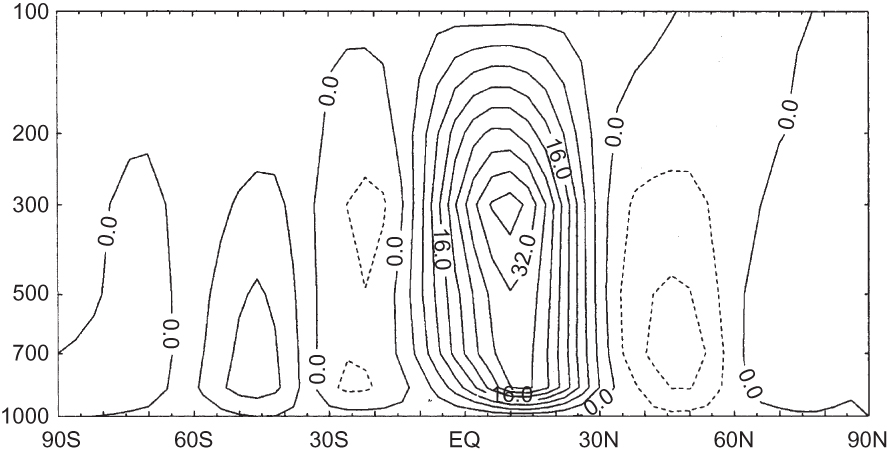
FIGURE 10.7 Streamfunction (units: 10² kg m-¹ s-¹) for the observed Eulerian mean meridional circulation for Northern Hemisphere winter. (Based on the data of Schubert et al., 1990).
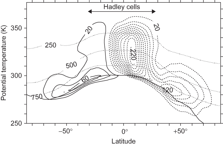
FIGURE 10.8 January time and zonal-mean isentropic mass flux streamfunction determined from ERA-40 reanalysis data 1980–2001). Streamfunction contours are shown every 20 × 109 kg s-¹, with implied clockwise circulation around negative values. Dotted lines show pressure surfaces and the solid lower curve is the median surface potential temperature. (Adapted from Schneider, 2006. Used with permission of Annual Reviews.)
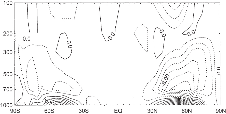
FIGURE 10.9 Eliassen–Palm flux divergence divided by the standard density ρ0 for Northern Hemisphere winter. (Units: ms-¹ day-¹.) (Based on the data of Schubert et al., 1990.)
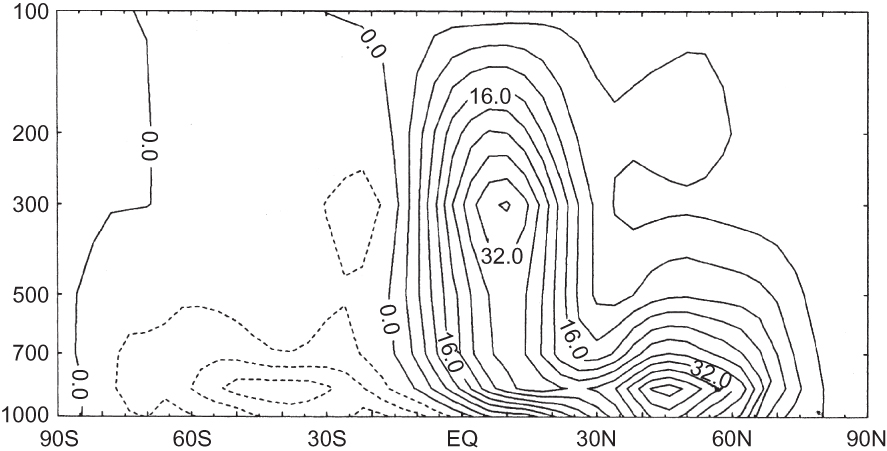
FIGURE 10.10 Residual mean meridional streamfunction (units: 10² kg m-¹ s-¹) for Northern Hemisphere winter. (Based on the data of Schubert et al., 1990.)
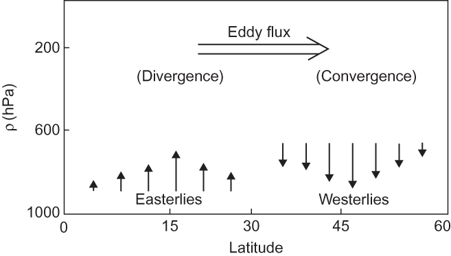
FIGURE 10.11 Schematic mean angular momentum budget for the atmosphere–Earth system.
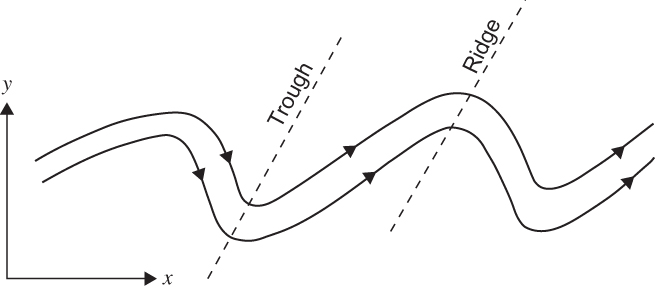
FIGURE 10.12 Schematic streamlines for a positive eddy momentum flux.
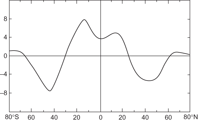
FIGURE 10.13 Latitudinal profile of the annual mean eastward torque (surface friction plus mountain torque) exerted on the atmosphere in units of 1018 m² kg s-². (Adapted from Oort and Peixoto, 1983.)
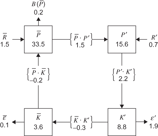
FIGURE 10.14 Observed mean energy cycle for the Northern Hemisphere. Numbers in squares are energy amounts in units of 105 Jm-². Numbers next to arrows are energy transformation rates in units of W m-². B(‾P) represents a net energy flux into the Southern Hemisphere. Other symbols are defined in the text. (Adapted from Oort and Peixoto, 1974. Copyright © American Geophysical Union. Used with permission.)
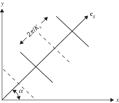
FIGURE 10.15 Stationary plane Rossby wave in a westerly flow. Ridges (solid lines) and troughs (dashed lines) are oriented at an angle α to the y axis; the group velocity relative to the ground, cg, is oriented at an angle α to the x axis. The wavelength is 2 π/Ks. (Adapted from Hoskins, 1983.)

FIGURE 10.16 Vorticity pattern generated on a sphere when a constant angular velocity westerly flow impinges on a circular forcing centered at 30°N and 45°W of the central point. Left to right, the response at 2, 4, and 6 days after the forcing is switched on. Five contour intervals correspond to the maximum vorticity response that would occur in 1 day if there were no wave propagation. Heavy lines correspond to zero contours. The pattern is drawn on a projection in which the sphere is viewed from infinity. (After Hoskins, 1983.)
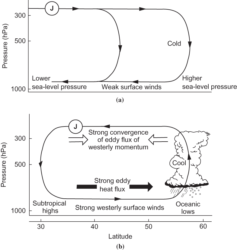
FIGURE 10.17 Meridional cross-sections showing the relationship between the time mean secondary meridional circulation (continuous thin lines with arrows) and the jet stream ("J") at locations (a) upstream and (b) downstream from the jet stream cores. (After Blackmon et al., 1977. Copyright © American Meteorological Society. Reprinted with permission.)
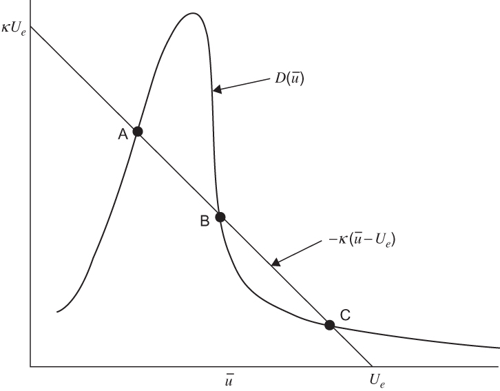
FIGURE 10.18 Schematic graphical solution for steady-state solutions of the Charney–DeVore model. (Adapted from Held, 1983.)
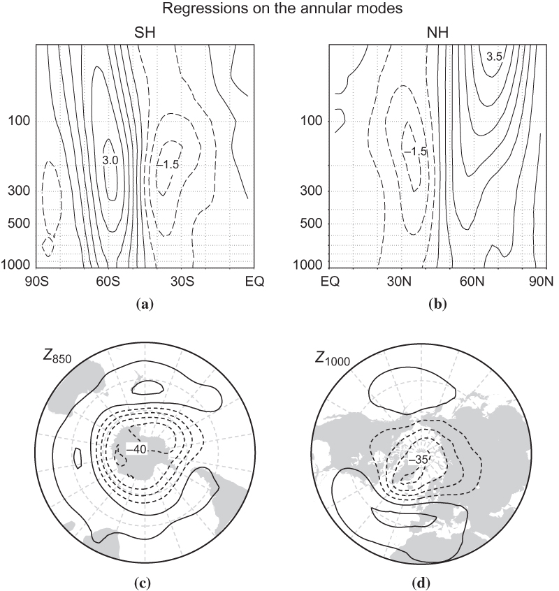
FIGURE 10.19 (a,b) Latitude–height cross-sections showing typical amplitudes of annular mode anomalies for mean-zonal wind (ordinate labels are pressure in hPa, contour interval 0:5ms-¹). (c,d) Lower tropospheric geopotential height (contour interval 10 m). The Southern Hemisphere (SH) is on the left and the Northern Hemisphere (NH) is on the right. Phase shown corresponds to the high-index state (strong polar vortices). The low-index state would have opposite signed anomalies. (After Thompson and Wallace, 2000. Copyright © American Meteorological Society. Reprinted with permission.)
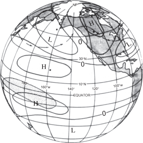
FIGURE 10.20 Pattern of middle and upper tropospheric height anomalies for Northern Hemisphere winter during an ENSO event in the tropical Pacific. The region of enhanced tropical precipitation is shown by shading. Arrows depict a 200-hPa streamline for the anomaly conditions. "H" and "L" designate anomaly highs and lows, respectively. The anomaly pattern propagates along a great circle path with an eastward component of group velocity, as predicted by stationary Rossby wave theory. (After Horel and Wallace, 1981. Copyright © American Meteorological Society. Reprinted with permission.)
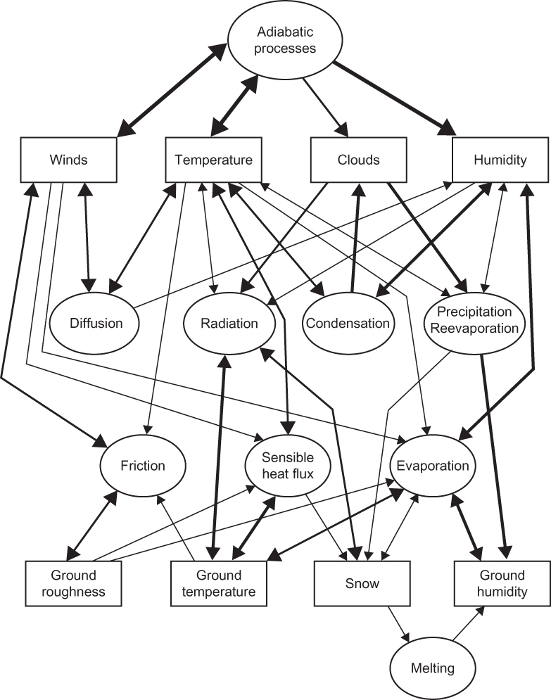
FIGURE 10.21 Schematic of processes commonly included in AGCMs and their interactions. The thickness of each arrow gives a rough indication of the importance of the interaction that a particular arrow represents. (After Simmons and Bengtsson, 1984. Copyright © Cambridge University Press. Used with permission.)
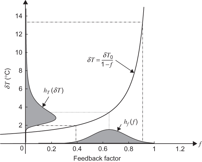
FIGURE 10.22 How (10.82) (solid curve) maps uncertainty in the feedback factor, f (abscissa) onto uncertainty in the temperature equilibrium change, δT (ordinate). Gray shading gives the probability density function, with a Gaussian distribution assumed for the feedback factor for purpose of illustration. The control equilibrium temperature change is taken to be 3°C. Dotted (dashed) lines show the mean (95% confidence interval) for the feedback factor. (Adapted with permission from Roe and Baker, 2007.)