Chapter 12
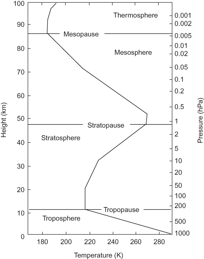
FIGURE 12.1 Midlatitude mean temperature profile. (Based on the U.S. Standard Atmosphere, 1976.)
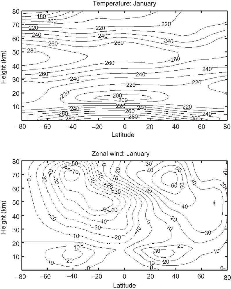
FIGURE 12.2 Observed monthly and zonally averaged temperature (K) and zonal wind (m s-¹) for January. (Based on Fleming et al., 1990.)
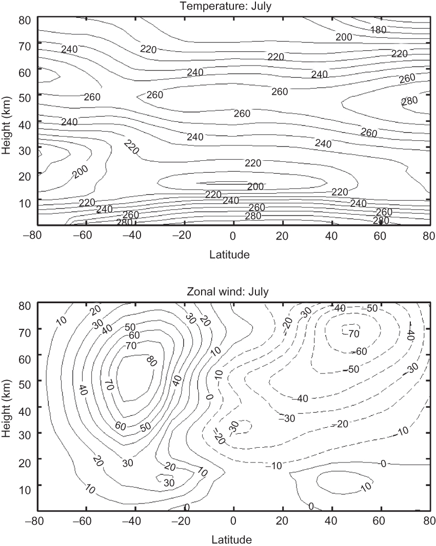
FIGURE 12.3 Observed monthly and zonally averaged temperature (K) and zonal wind (m s-¹) for July. (Based on Fleming et al., 1990.)
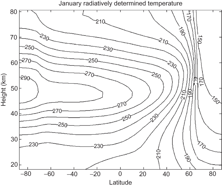
FIGURE 12.4 Radiatively determined middle atmosphere temperature distribution (K) for northern winter soltice from a radiative model that is time-marched through an annual cycle. Realistic tropospheric temperatures and cloudiness are used to determine the upward radiative flux at the tropopause. (Based on Shine, 1987.)
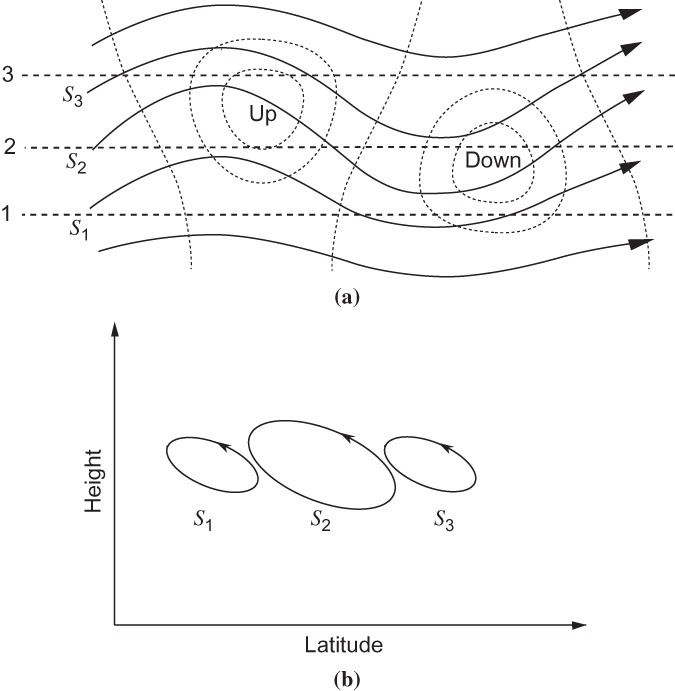
FIGURE 12.5 Parcel motions for an adiabatic planetary wave in a westerly zonal flow. (a) Solid lines labeled S1, S2, and S3 are parcel trajectories, heavy dashed lines are latitude circles, and light dashed lines are contours of the vertical velocity field. (b) Projection of parcel oscillations on the meridional plane.
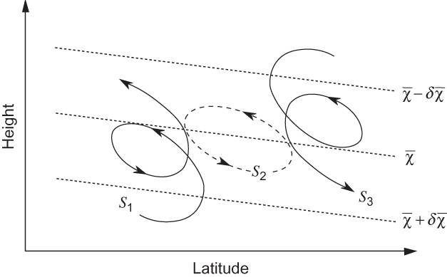
FIGURE 12.6 Projections of parcel motions on the meridional plane for planetary waves in westerlies with diabatic heating at low latitudes and diabatic cooling at high latitudes. Thin dashed lines show tilting of isosurfaces of tracer mixing ratio due to transport by the diabatic circulation.
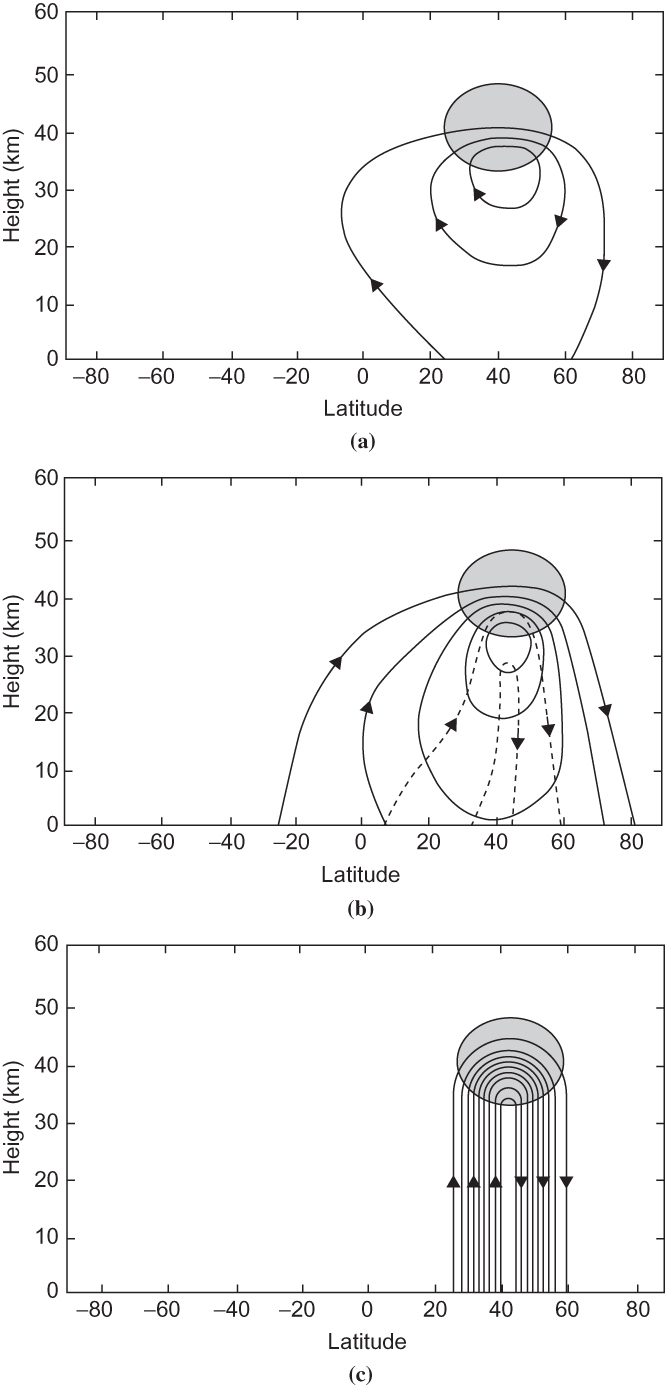
FIGURE 12.7 Response of the zonally symmetric circulation to a westward force applied in the shaded region. Contours are streamlines of the TEM meridional circulation, with the same contour interval used in each panel. (a) Adiabatic response for high-frequency forcing. (b) Response for annual frequency forcing and 20-day radiative damping timescale; solid and dashed contours show the response that is in phase and 90° out of phase, respectively, with the forcing. (c) Response to steady-state forcing. (After Holton et al., 1995. Used with permission of American Geophysical Union.)
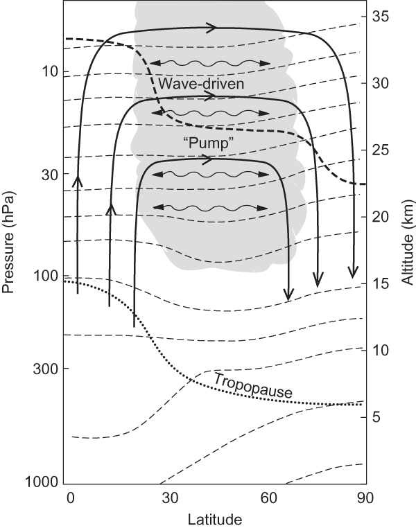
FIGURE 12.8 Schematic cross-section of the wave-driven circulation in the middle atmosphere and its role in transport. Thin dashed lines denote potential temperature surfaces. Dotted line is the tropopause. Solid lines are contours of the TEM meridional circulation driven by the wave-induced forcing (shaded region). Wavy double-headed arrows denote meridional transport and mixing by eddy motions. Heavy dashed line shows an isopleth of mixing ratio for a long-lived tracer.
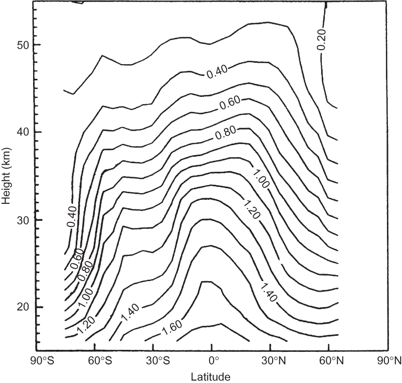
FIGURE 12.9 October zonal mean cross-section of methane (ppmv) from observations by the HALOE on the UARS. Note the strong vertical stratification due to photochemical destruction in the stratosphere. The upward-bulging mixing ratio isopleths in the equatorial region are evidence of upward mass flow in the equatorial region, whereas the downward-sloping isopleths in high latitudes are evidence of subsidence in the polar regions. The region of flattened isopleths in the midlatitudes of the Southern Hemisphere is evidence for quasi-adiabatic wave transport due to wintertime planetary wave activity. (After Norton, 2003.)
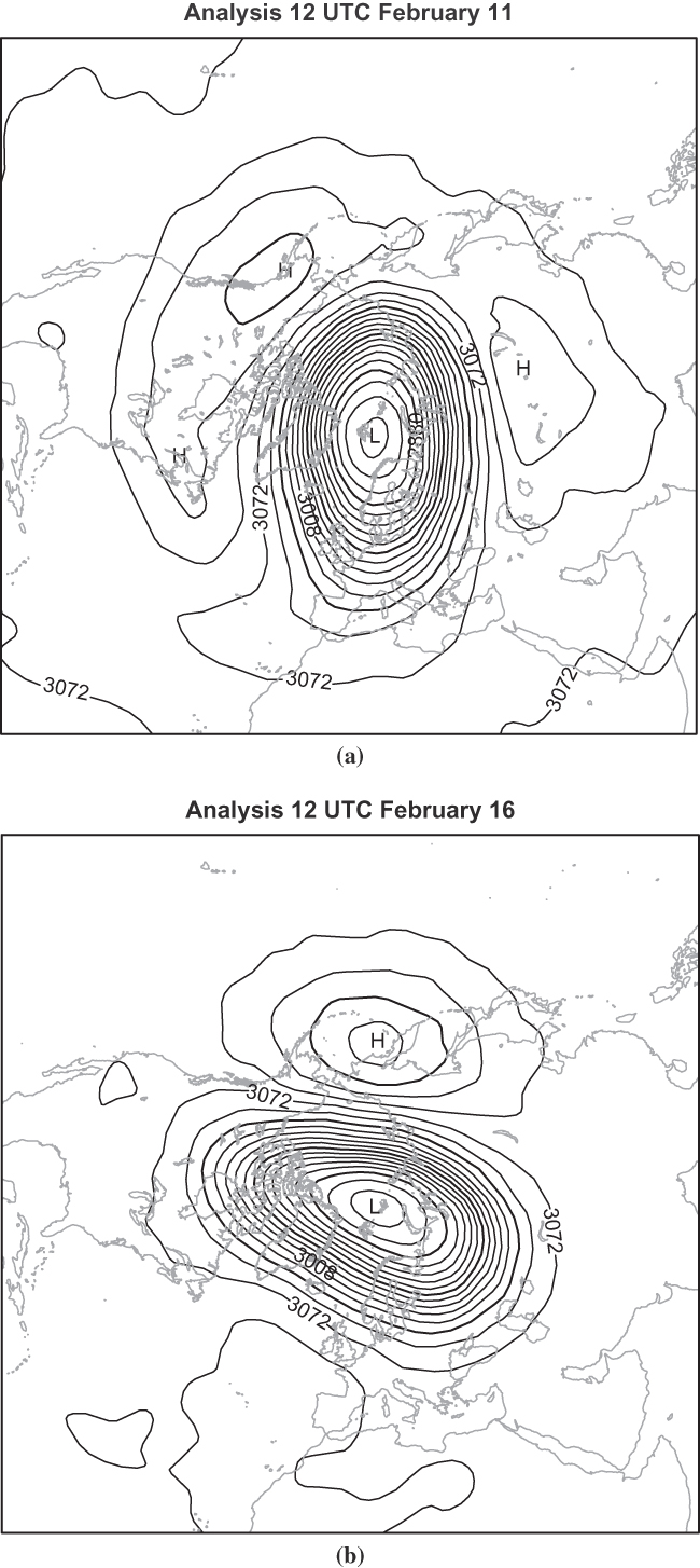
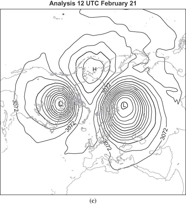
FIGURE 12.10 10-hPa geopotential height analyses for days in 1979: February 11 (a), February 16 (b), and February 21 (c) at 12 UTC, showing breakdown of the polar vortex associated with a wave number 2’s sudden stratospheric warming. Contour interval: 16 dam. (Analysis from ERA-40 reanalysis courtesy of the European Centre for Medium-Range Weather Forecasts.)
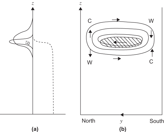
FIGURE 12.11 Schematic of transient wave, mean–flow interactions occurring during a stratospheric warming. (a) Height profiles of EP flux (dashed line), EP flux divergence (heavy line), and mean zonal flow acceleration (thin line); z0 is the height reached by the leading edge of the wave packet at the time pictured. (b) Latitude–height cross-section showing region where the EP flux is convergent (hatching), contours of induced zonal acceleration (lines), and induced residual circulation (arrows). Regions of warming (W) and cooling (C) are also shown. (From Andrews et al., 1987.)
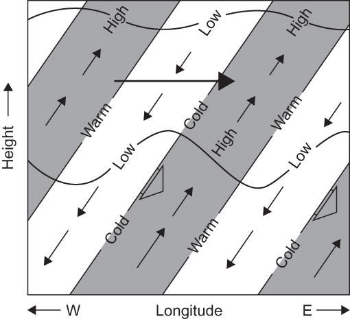
FIGURE 12.12 Longitude–height section along the equator showing pressure, temperature, and wind perturbations for a thermally damped Kelvin wave. Heavy wavy lines indicate material lines; short black arrows show phase propagation. Areas of high pressure are shaded. Length of the small thin arrows is proportional to the wave amplitude, which decreases with height due to damping. The large shaded arrow indicates the net mean flow acceleration due to the wave stress divergence.
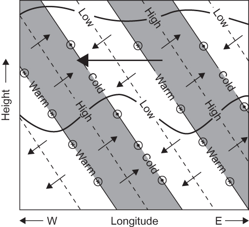
FIGURE 12.13 Longitude–height section along a latitude circle north of the equator showing pressure, temperature, and wind perturbations for a thermally damped Rossby–gravity wave. Areas of high pressure are shaded. Small arrows indicate zonal and vertical wind perturbations with length proportional to the wave amplitude. Meridional wind perturbations are shown by arrows pointed into the page (northward) and out of the page (southward). The large shaded arrow indicates the net mean flow acceleration due to the wave stress divergence.
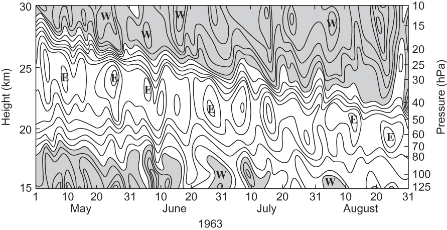
FIGURE 12.14 Time–height section of zonal wind at Canton Island (3°S). Isotachs at intervals of 5 m s-¹. Westerlies are shaded. (Courtesy of J. M. Wallace and V. E. Kousky.)
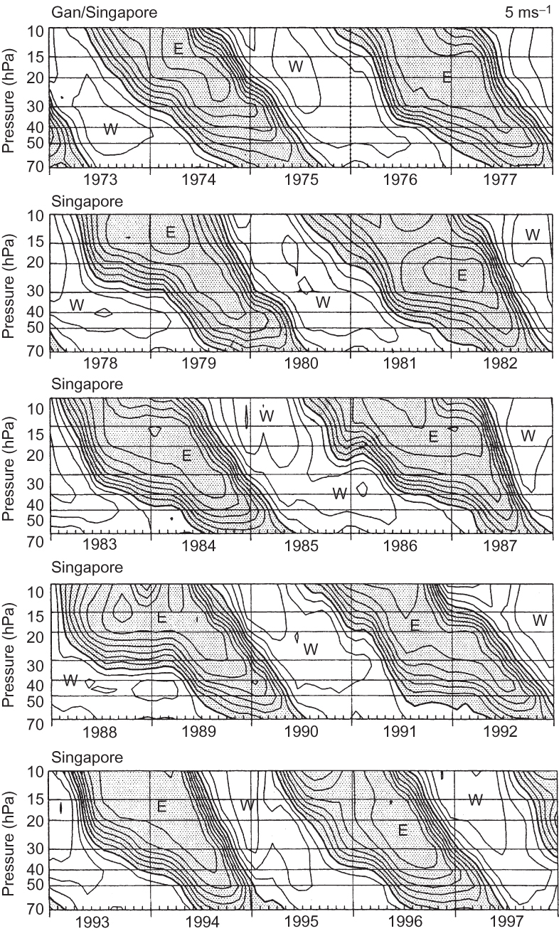
FIGURE 12.15 Time–height section of departure of monthly mean zonal winds (m s-¹) for each month from the long-term average for that month at equatorial stations. Note the alternating downward-propagating westerly (W) and easterly (E) regimes. (After Dunkerton, 2003. Data provided by B. Naujokat.)
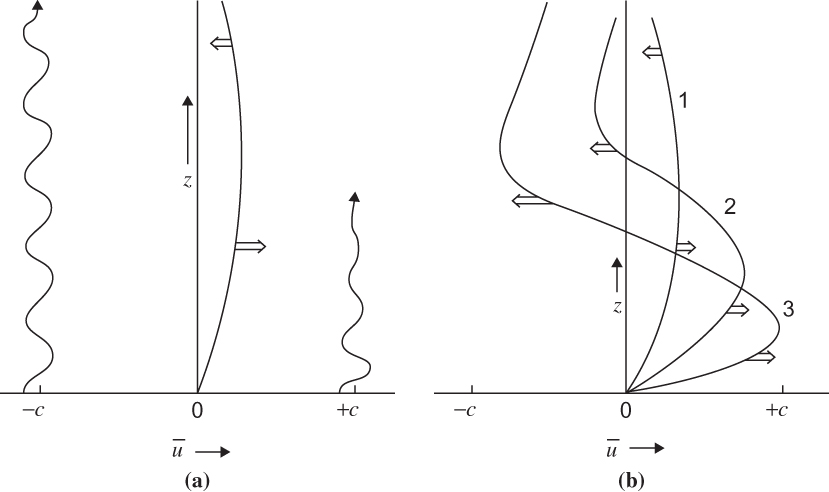
FIGURE 12.16 Schematic representation of wave-driven accelerations that lead to the zonal wind QBO. Eastward- and westward-propagating gravity waves of phase speeds +c and –c, respectively, propagate upward and are dissipated at rates dependent on the Doppler-shifted frequency. (a) Initial weak westerly current selectively damps the eastward-propagating wave and leads to westerly acceleration at lower levels and easterly acceleration at higher levels. (b) Descending westerly shear zones block penetration of eastward-propagating waves, whereas westward-propagating waves produce descending easterlies aloft. Broad arrows show locations and direction of maxima in mean wind acceleration. Wavy lines indicate relative penetration of waves. (After Plumb, 1982.)
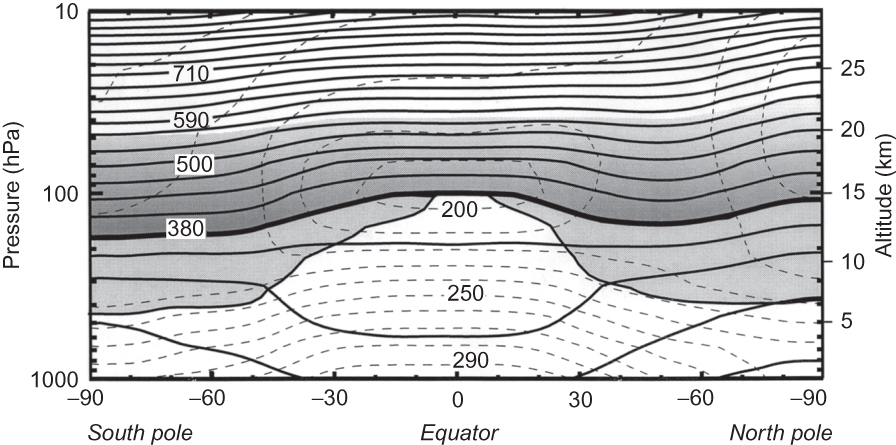
FIGURE 12.17 Latitude–height section showing January mean potential temperature surfaces (solid contours) and temperature (dashed contours). Heavy line shows the 380-K θ surface, above which all θ surfaces lie completely in the middle atmosphere. The light shaded region below the 380 K surface is the lowermost stratosphere, where Θ surfaces span the tropopause (shown by the line bounding the lower side of the shaded region). (Courtesy of C. Appenzeller.)