Chapter 13
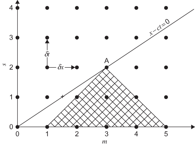
FIGURE 13.1 Grid in x – t space showing the domain of dependence of the explicit finite-difference solution at m = 3 and s = 2 for the one-dimensional linear advection equation. Solid circles show grid points. The sloping line is a characteristic curve along which q(x, t) = q(0, 0), and the “+” shows an interpolated point for the semi-Lagrangian differencing scheme. In this example the leapfrog scheme is unstable because the finite difference solution at point A does not depend on q(0, 0).
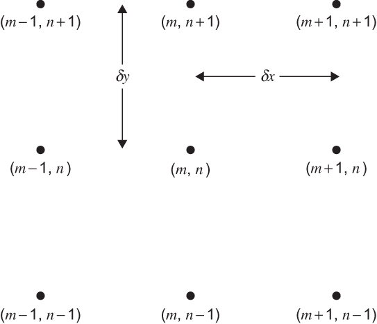
FIGURE 13.2 Portion of a two-dimensional (x, y) grid mesh for solution of the barotropic vorticity equation.
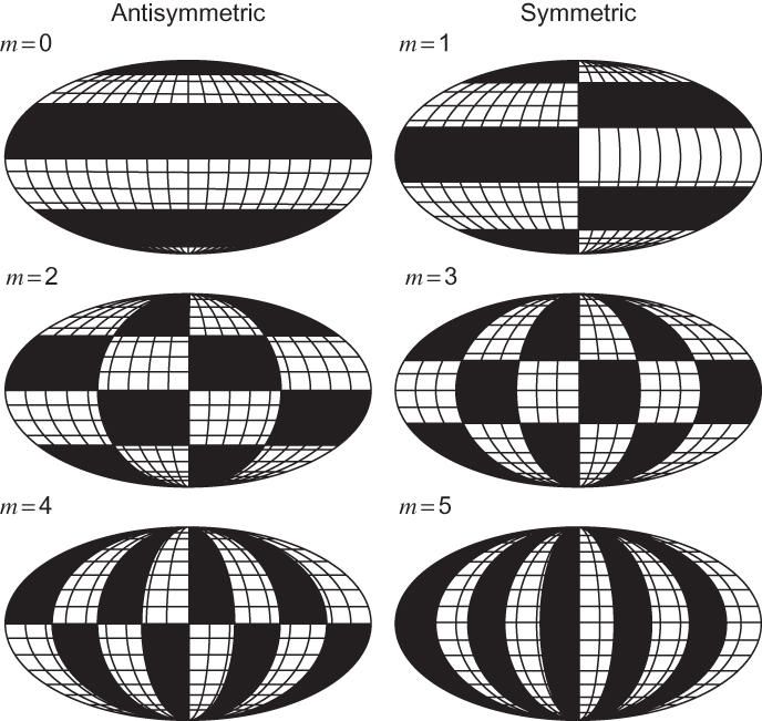
FIGURE 13.3 Patterns of positive and negative regions for the spherical harmonic functions with n = 5 and m = 0, 1, 2, 3, 4, 5. (After Washington and Parkinson, 1986; adapted from Baer, 1972. Copyright © American Meteorological Society. Reprinted with permission.)
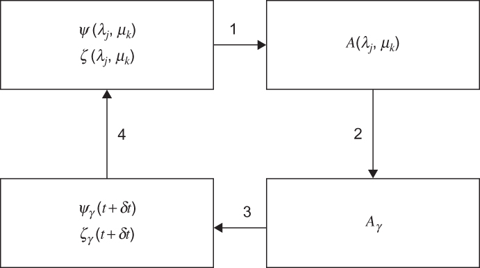
FIGURE 13.4 Steps in the prediction cycle for the spectral transform method of solution of the barotropic vorticity equation.
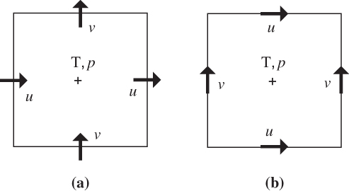
FIGURE 13.5 Horizontal grid staggering schemes for the Arakawa-C (a) and Arakawa-D (b) grids. Thermodynamic (T, p) and other scalar fields are located at the center of the grid cell; horizontal velocity components u and v are located along the grid edge.
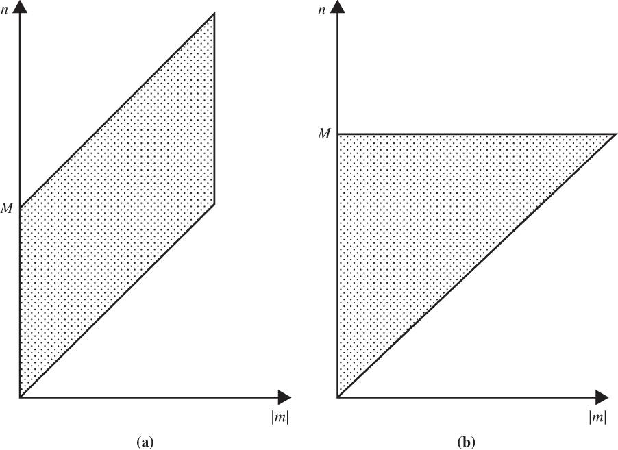
FIGURE 13.6 Regions of wave number space (n, m) in which spectral components are retained for the rhomboidal truncation (a) and triangular truncation (b). (After Simmons and Bengtsson, 1984. Used with permission.)
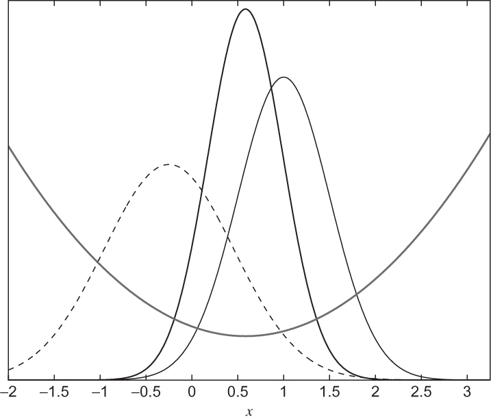
FIGURE 13.7 Data assimilation for scalar variable x assuming Gaussian error statistics. Prior estimate xb, given by the dashed line, has mean –0.25 and variance 0.5. Observation y, given by the thin solid line, has mean 1.0 and variance 0.25. The analysis, xa, given by the thick solid line, has mean 0.58 and variance 0.17. The parabolic gray curve denotes the cost function, J, which takes a minimum at the mean value of xa.
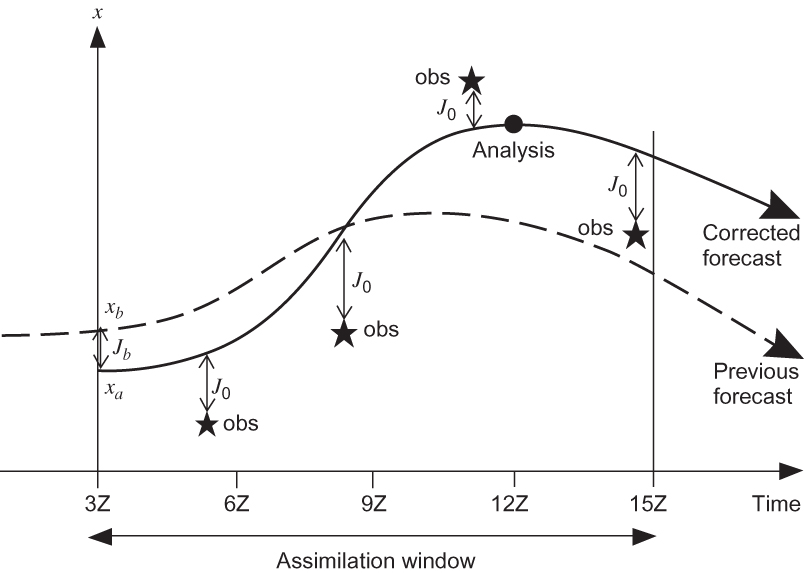
FIGURE 13.8 ECMWF data assimilation process. The vertical axis indicates the value of an atmospheric field variable. The curve labeled xb is the first guess or "background" field, and xa is the analysis field. Jb indicates the misfit between the background and analysis fields. Stars indicate the observations, and J0 designates the “cost function,” a measure of the misfit between the observations and the analysis, which along with Jb is minimized to produce the best estimate of the state of the atmosphere at the analysis time (Courtesy ECMWF.)
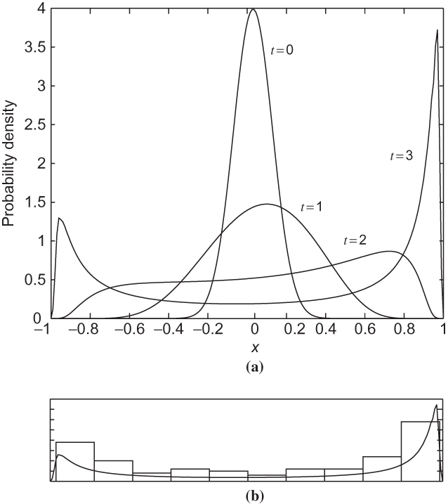
FIGURE 13.9 Time evolution of an initially Gaussian probability density function subject to the dynamics in (13.67) from numerically solving the Liouville equation (a). Populating a 100-member ensemble by randomly sampling from the initial probability density function, and solving (13.67) for the state at t = 3—summarized by a histogram in (b)—provides an estimate of the solution of the Liouville equation (solid line).
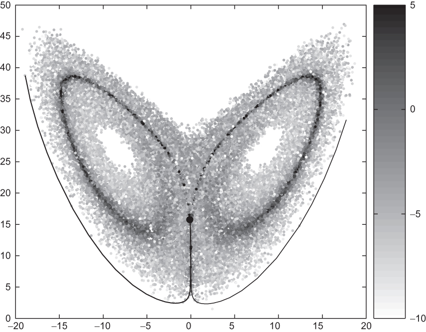
FIGURE 13.10 Sensitivity of forecasts to initial condition errors for the Lorenz (1963) attractor (forecasts are one time unit long). The natural logarithm of the errors is depicted in gray-scale, with darker gray indicating points that yield forecasts with larger errors. Solutions for the most sensitive location are given by lines.
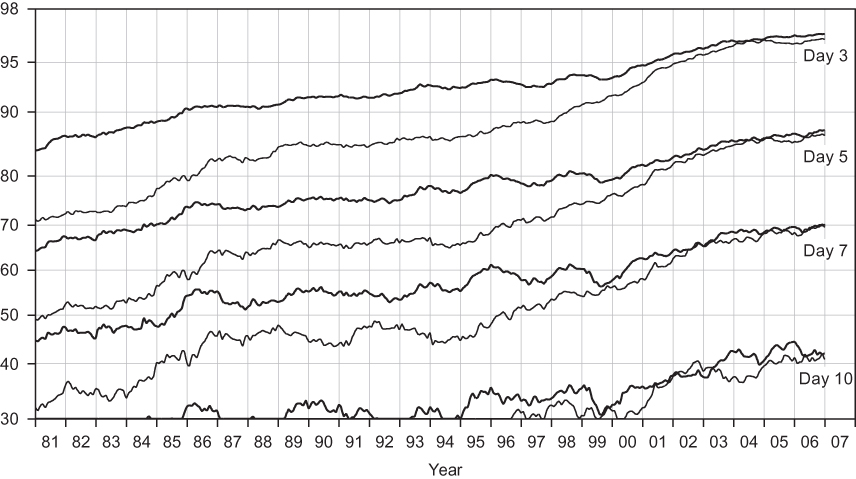
FIGURE 13.11 Anomaly correlation of 500-hPa height for 3-, 5-, 7-, and 10-day forecasts for the ECMWF operational model as a function of year. Thick and thin lines correspond to Northern and Southern Hemispheres, respectively. Note that the difference in skill between the two hemispheres has nearly disappeared in the last decade, a result of the successful assimilation of satellite data. (Courtesy ECMWF.)